Concepts

In Altaxo a 2D graph consists of at least one layer, the root layer (RL). The root layer represents the outer boundaries of the graph. By changing the size of the root layer, you change the size of the graph. The root layer usually contains child items. In most cases there is only one child item, an additional layer, namely the plot layer L0.

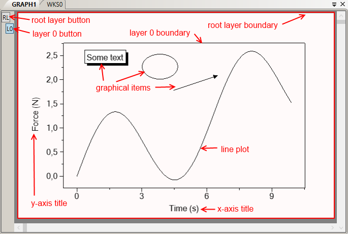
The figure above shows the screenshot of a graph window in Altaxo. All red items are for illustration only and do not belong to the graph. The area inside the red frame designates the root layer. You can change the properties of the root layer by clicking the root layer button (the button labeled 'RL' in the upper left corner of the graph window).

The root layer shown here has exactly one child layer, namely the layer 'L0'. In the figure above, the area of layer 'L0' is indicated by the black frame. You can change the properties of layer L0 by clicking the button labeled 'L0' (below the root layer button in the upper left corner of the graph window). The frame of layer L0 is the inner rectangle.

Layer 0 has multiple child items: some graphical items (text, ellipse, arrow), a line plot, the x-axis title, the y-axis title, and axis lines, axis ticks and axis labels. Please note that some of the child items of layer 0 (e.g. the axis titles) are located outside the frame of layer 0. Nevertheless they belong to layer 0.

When you add graphical items to the graph, it is essential to care about to which layer you add the new items. There is always exactly one active layer, the layer to which new items will be added. In the figure above, layer 0 (L0) is the active layer, indicated by the blue background of the layer 0 button.

Altaxo distinguishes between scales and axes. The two words seem to be similar, so what is the difference?

The difference is that while an x-y plot layer has exactly two scales, namely the x scale and the y scale, it normally has multiple axes. The axes are the graphical representation of the scales. For instance, usually the x scale has a graphical representation at the bottom of the plot layer, but can also have a graphical representation at the top of the layer or even in the middle of the layer.

The scale is responsible for converting the physical values (your data values) into logical values that designate the position along the scale. The logical value 0 represents the origin of the scale, the logical value of 1 represents the end of the scale. Thus a pair of physical values (x,y) can be converted to a pair of logical values (lx, ly), which finally designate a specific position onto the plot layer. Different scales (linear, logarithmic etc.) are nothing more than different conversion laws between physical values and logical values. Properties of a scale are usually the physical values at the origin and the end of the scale. That`s all. But there are two other properties associated with a scale: First, there has to be some information how the scale behaves if the underlying data changed. Should it rescale to include all of the data? Should the boundaries of the scale be fixed? Therefore, the boundary conditions determine the behavior of the scale if the underlying data are changed or if the user tries to zoom the scale. Second, there are axis ticks. Here we have a compromise: ticks normally belong to the axis, not to the scale, as they mainly influence the graphical representation of the scale. But in Altaxo, the ticks can also influence the scale itself, specifically its origin and end, because the user can choose to let the scale start and/or end at either a major or a minor tick. Thus the tick spacing influences the physical values of the origin and then end of the scale. Summarizing, a scale is associated with one boundary condition and one tick spacing.

In contrast, an axis is one graphical representation of the scale. It has properties like the position of the axis (e.g. bottom, top, right or left), the color of the axis line and ticks, the width of the line, the font family and font size of the axis labels, and so on. Since the tick spacing is also an important property of the axis, you can override the tick spacing that is already associated with the underlying scale. Thus, for the same underlying scale, you can have different axes with different tick spacings.

Next section: Creating a graph