Spectroscopy

Spectra can be imported into Altaxo in various formats:

• Ascii (.txt; .dat; .csv)

• Galactic SPC (.spc)

• Jcamp-DX (.dx; .jdx)

• Renishaw (.wdf)

Some of these formats, e.g. Galactic SPC files, can contain more than one spectrum per file. In this case, all contained spectra are imported from the file.

In order to import one or multiple spectra, first create an empty worksheet. Either use the menu File → New → Worksheet, or use the toolbar button .

The next action depends on the file format to import:

• For Ascii files, you can use the toolbar button for import, or the menu File → Import → Ascii. If multiple spectra needs to be imported into one worksheet (for instance for chemometric analysis), use File → Import → Ascii (all into a single worksheet). Select all files that should be imported. Further information can be found in the section "Importing ASCII data".

• For all other files, use the menus File → Import → Galactic SPC files, File → Import → JCamp-DX files, or File → Import → Renishaw .wdf files. Here too, you can select multiple files.

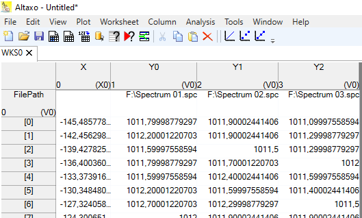
Fig. 1: Example of a worksheet after import of three .spc files. Note that the first "row" is a property, designating the original file name of the column. Furthermore, all three spectra have a common x-column named "X".

After successful import of the data, the worksheet contains a data source that holds all information of the import: which file(s) were imported, and which options were used for import. You can open the dialog to edit these data by clicking on the question mark in the toolbar. If you simple want to reimport the data without changing the file names or the options (e.g. when you have accidentally deleted your data), you can click on the Requery table data source button in the toolbar.

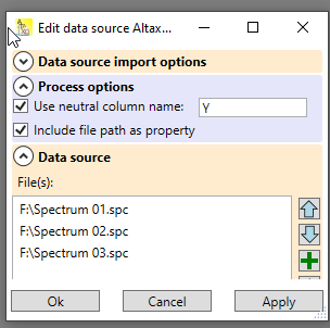
Fig. 2: Data source dialog of the example worksheet used above. In the options, the name of the columns (which starts now with "Y") can be changed. The data source contains the three file names of the imported spectra.

For many spectra that are output by a spectrometer, spectral preprocessing might be necessary prior to the further evaluation of the spectra, for instance by chemometric methods.

Spectral preprocessing includes:

• removal of cosmic spikes (excitation of single spectrometer pixels by cosmic radiation)

• x-axis calibration (wavelength correction by a calibration)

• y-axis calibration (intensity correction by a calibration)

• baseline removal

• smoothing

• cropping (in order to drop uninteresting areas of the spectrum)

• resampling (changing the x-axis resolution)

• normalization

Altaxo features a spectral preprocessing pipeline, implementing the steps described above.

Usage

Import one or multiple spectra. If the spectra should be treated with the same preprocessing steps, it is preferable to import them into a single worksheet.

Select all columns in that worksheet which contains the intensities. Do not select the x-columns containing the wavelengths.

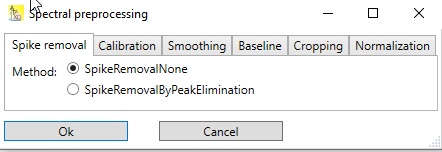
Use the menu Analysis → Spectroscopy → Preprocess to open the preprocessing dialog. The preprocessing dialog contains multiple tabs for the preprocessing steps described above. Each tab allows the selection of different preprocessing methods for its topic. Each tab contains a 'None' method, which essentially means, that when selected, nothing is being done in that step.

Fig.1: Spectral preprocessing dialog with tabs for various steps

After selection of the required methods and pressing OK, a new worksheet is created, which contains the preprocessed spectra. The name of the new worksheet is the name of the original worksheet with the string _preprocessed appended to it.

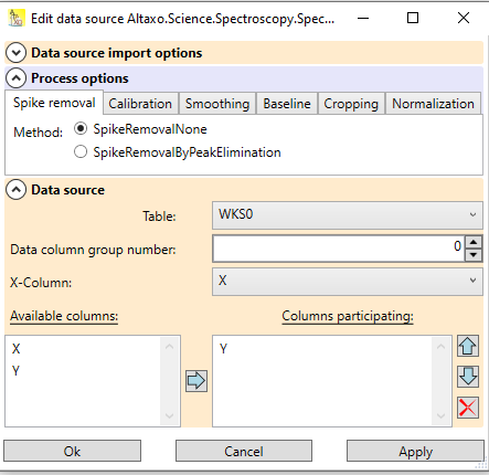
The newly created table contains a data source for the preprocessing. The data source remembers where the data of the preprocessing came from, and which preprocessing steps have been performed. If the result of the preprocessing is not satisfactory, the data source can be opened by clicking on the question mark in the toolbar. Using this dialog, the preprocessing steps can be changed, or data can be added or removed.

Fig.2: Data source of the worksheet containing the preprocessed spectra. The expander in the center contains the preprocessing options; the expander at the bottom contains the information about the origin of the data to process.

Additionally, when the original data have changed, you can re-apply the preprocessing by clicking on the Requery table data source button in the toolbar.

In the following sections, the various preprocessing steps are described in more detail.

Spike removal

Some spectrometers, for instance Raman spectrometers, need to detect very low intensities. On those spectrometers, radiation coming from cosmic particles and from other sources can hit a pixel of the detector. This will increase the counts of this pixel, often much more than the wanted signal. The excitation is limited to this pixel, or to this and very few neighboring pixels, and thus cause a sharp peak in the spectrum.

Those peaks spoil the further preprocessing of the spectrum, e.g. smoothing, base line correction, and normalization, and therefore needs to be eliminated.

Currently, there is only one method in the Spike removal tab. It is

SpikeRemovalByPeakElimination

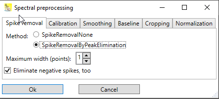
This method has only two parameters (see Fig.1):

1. Maximum width in points. The maximum width of the spikes (in pixel) that should be eliminated. Often, a width of 1 is sufficient to remove cosmic spikes. If neighboring pixels are also affected, the width parameter can be increased. Please be aware that this increases the risk that wanted peaks are eliminated, too.

2. Eliminate negative spikes: For background removal, often a dark spectrum is subtracted from the measured spectrum. If the dark spectrum contains cosmic spikes, then these will appear in the resulting spectrum as negative spikes. If negative spikes occur in the spectrum, the checkbox should be checked. If not removed, negative spikes will spoil mainly the baseline correction step, and the normalization step.

Fig. 1: Dialog for the SpikeRemovalByPeakElimination step

Calibration

This tab allows you to change the x-axis of your spectrum from an uncalibrated x-axis to a calibrated x-axis.

The prerequisite for this is the presence of a table which contains a valid x-calibration. Such a table can be created for instance for Raman instruments using a spectrum of a Neon lamp and a Raman spectrum of silicon (see Raman calibration with Neon and Silicon).

Using this calibration table to change the x-axis of the spectrum is straightforward (see Fig. 1): In the combobox all tables that contain a valid x-calibration are listed, and the most recent calibration is preselected. Simply choose the table that contains the calibration you want to apply.

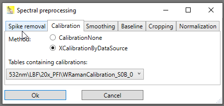
Fig. 1: Calibration tab. The combobox lists all tables containing calibrations, and the most recent calibration is preselected.

Smoothing

The smoothing step will apply some smoothing algorithm to the spectral data in order to reduce the noise level.

Currently, only one smoothing method is implemented:

Smoothing by Savitzky-Golay

The method uses the Savitzky-Golay method to smooth a signal. Basically, it is a local polynomial fit, of which the center fit value is used as replacement for the original point. As an additional option, not only the center fit value, but also the derivative at that point can be used (but note that the x-values are not used to calculate the derivative value).

Savitzky-Golay has the following options:

• Number of points: The number of points for the local fit. The more points, the smoother the result, but the more the original shape of the spectrum is changed.

• Polynomail order: The polynomial order of the fit. The default value of 2 means that a quadratic fit is applied.

• Derivative order: The default value of 0 means the central fit function value is used to replace the original point. A value of 1 means the first derivative is used, etc. Note that the result is not the true derivative, since the x-values are not used for evaluation of the derivative (the space between the points is assumed to be 1).

Baseline

Baseline correction is essential, because some of the subsequent methods, for instance some of the peak fitting methods, assume that the baseline was corrected before, so that the base of the peaks can be assumed to be zero.

Different baseline correction methods exist, but non of them is waterproof. The reason is simply, that there is information missing. Assume your entire spectrum consists of massive overlapping peaks, there is no way to determine a baseline, because each spectral point has intensity from at least one peak.

The methods described below therefore assime that at least in some regions of the spectrum there are no neighboring peaks, and the intensity in those regions is at its base level.

AirPLS, ALS, ArPLS

These are methods based on diffusion equations. Thus all methods exhibit a diffusion constant lamda. The higher lambda is, the more flat is the resulting baseline. This group of methods is especially well suited if the spectrum exhibits a high noise level, but require some manual adjustment of the parameters by trial-and-error.

References:
[1] Zhang ZM, Chen S, Liang YZ. "Baseline correction using adaptive iteratively reweighted penalized least squares", Analyst. 2010 May; 135(5):1138-46, Epub 2010 Feb 19. PMID: 20419267, https://doi.org/10.1039/b922045c

[2] Sung-June Baek, Aaron Park, Young-Jin Ahn and Jaebum Choo, "Baseline correction using asymmetrically reweighted penalized least squares smoothing", Analyst, 2015, 140, 250-257, https://doi.org/10.1039/C4AN01061B

[3] Paul H.C. Eilers, Hans F.M. Boelens, "Baseline Correction with Asymmetric Least Squares Smoothing", October 21, 2005

PolynomialDetrending

Strictly speaking, this is not a method to guess the baseline, since the entire spectrum is used for evaluation. The method evaluates a polynomial fit of user-defined order of the entire spectrum. The resulting polynomial is then used as the baseline. The method may perform good if only very few and narrow peaks exist in the spectrum. The method requires a user defined parameter: the detrending order. Choose a value of

• 0 for subtracting a constant (in this case, the mean of the y-values)

• 1 for subtracting a linear slope

• 2 for subtracting a quadratic function

SNIP (linear and loglog)

This implements the SNIP algorithm. Basically, the method spans a line between two spectral points. The width of the line is defined by the user, but must be an odd number of spectral points. The resulting baseline point is then either used from the spectrum (if the center of the line lies above the spectrum), or from the center of the line (if the center of the line lies below the spectrum). This is repeated for a fixed number of iterations.

SNIPLinear is using the original spectral y-values, whereas SNIPLogLog first takes twice the logarithm of the y-values, which presumes that the y-values are all positive.

The following options are available:

• Half width: the half of the (width of the line described above minus 1). Thus, a value of 1 means the width of the line is 3 points; a value of 10 means a line width of 21 points. The half width can also be entered in units of the x-axis of the spectrum. The value of the half width should be at least that of the full (!) width of the broadest peak in the spectrum.

• Number of iterations: The default value of 40 is appropriate for most applications.

References:

[1] C.G. Ryan, E. Clayton, W.L. Griffin, S.H. Sie, D.R. Cousens, "SNIP, a statistics-sensitive background treatment for the quantitative analysis of PIXE spectra in geoscience applications", Nuclear Instruments and Methods in Physics Research Section B: Beam Interactions with Materials and Atoms, Volume 34, Issue 3, 1988, pp. 396-402, ISSN 0168-583X, https://doi.org/10.1016/0168-583X(88)90063-8

Cropping

Cropping selects only the interesting part of the spectrum.

The different methods are:

Cropping by indices

Here, the minimal index and the maximal index of the points that should be includes in the spectrum are given. Note that indexing is zero based: If the first point should be included, the minimal index has to be set to 0. Negative indices are allowed too, designating then the offset from the point after the last point. Thus a value of -1 represents the last point, -2 the point before the last point etc.

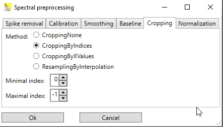
Fig. 1: Dialog for cropping by indices. Because here the minimal index is 0, meaning the first point, and the maximal index is -1, meaning the last point, the entire spectrum is included (which is the same as choosing CroppingNone)

Cropping by x-values

The range of the spectrum that should be included is given in units of the x-axis of the spectrum. By default, the minimal value is -∞ and the maximal value ∞, meaning that the entire spectrum is included, but minimal value and maximal value can be adjusted.

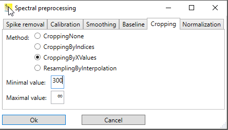
Fig. 2: Dialog for cropping a spectrum by providing the minimum and maximum x-value. Here, the minimum x-value is given as 300, whereas the maximum value is left at infinity.

Resampling by interpolation

This method combines cropping with a resampling of the x-axis. Resampling means changing the x-axis points to new values, thereby enhancing the x-value spacing or decreasing it. It is often used to make the x-axis values equidistant again (for instance after applying x-calibration). In order to get the y-values at new x-values, the values needs to be interpolated between to existing points.

This method has a bunch of different options:

• Interpolation method: Choose a interpolation method. Different types of splines are available, even smoothing splines, which require additional parameters to be entered.

• Sampling: Basically, the start value, the end value and the number of points are needed. But the dialog allows to choose between different options here:

  • specifying the x-values by start, end and count (number of points)

  • specifying the x-values by start, end and step value

  • specifying the x-values by start, step value and count

  • specifying the x-values by end, count and step value There is a preview box that shows the first three and the last three x-values that would be generated by your choice.

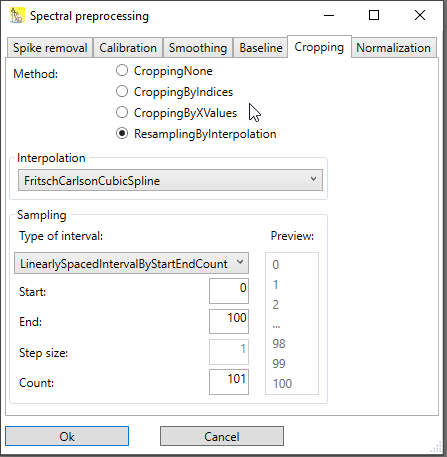
Fig. 3: Dialog for resampling by interpolation.

Normalization

Normalization scales the y-values of the spectrum according to different algorithms.

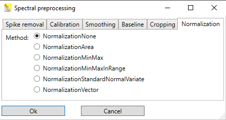
Fig.1 Normalization tab with different options for normalization.

The different options for normalization are described in the following sections.

NormalizationArea

Executes area normalization:

in which is the minimal y-value and is the average of all y-values. This results in a spectrum for which:

• the minimal y-value is 0

• the sum of all y-values is 1

NormalizationMinMax

Executes min-max normalization:

in which and are the minimal and the maximal y-values, respectively. This results in a spectrum for which:

• the minimal y-value is 0

• the maximal y-value is 1

NormalizationMinMaxInRange

Executes min-max normalization, but for determination of and , only a user-defined region of the spectrum is used:

in which and are the minimal and the maximal y-values in the user defined region, respectively. This results in a spectrum for which:

• the minimal y-value is 0 in the user defined region

• the maximal y-value is 1 in the user defined region

• the y-values outside the user defined region are affected, too, but can be less than 0 or greater than 1

Use this normalization technique e.g. if there is a well defined reference peak, and the rest of the spectrum should be scaled to that reference peak. In this case, the user-defined region should include the maximum of the reference peak, but also the base(s) of that peak.

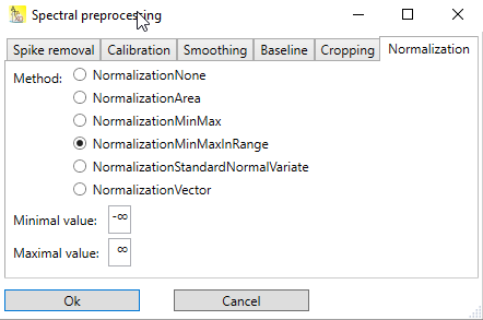
Fig. 2: The normalization method NormalizationMinMaxInRange requires the input of the range of x-values of the user defined region.

NormalizationStandardNormalVariate

Executes SNV (standard normal variate) normalization:

in which is the average of all y-values and is the standard deviation of the y-values.

This results in a spectrum for which:

• the sum of all y-values and the average is 0

• the standard deviation of the y-values is 1

NormalizationVector

Executes vector normalization:

in which is the L2 norm of the y-values, i.e.

This results in a spectrum for which:

• the L2 norm of the y-values is 1

It may be interesting to know the positions, widths, and heights (or areas) of the peaks of a spectrum.

Peak searching and fitting usually consist of three steps (there is one exception, which will be described later):

1. a peak searching algorithm searches for peaks and outputs the approximate positions, widths and heights of the found peaks

2. the approximate positions, widths and heights that are the result of the peak searching step are used as initial values for peak fitting. Then a peak fitting algorithm evaluates these values with a higher accuracy. Other quantities, like the area under the peak, can be output, too.

3. Output the results in a new worksheet, and (optionally) plot the fit curve together with the original spectral data.

Altaxo features a peak searching and fitting pipeline, implementing the two steps described above.

Usage

Import one or multiple spectra. If the spectra should be treated with the same steps, it is preferable to import them into a single worksheet.

Select all columns in that worksheet which contains the spectral intensities. Do not select the x-columns containing the wavelengths.

Use the menu Analysis → Spectroscopy → PeakFinding+Fitting to open the peak finding+fitting dialog. The dialog contains multiple tabs. The first tabs are for the preprocessing steps described in section Spectral Preprocessing. The last three tabs contain options for the search step, the fit step, and the output step described above.

Fig.1: Spectral preprocessing dialog with three additional steps for peak searching, fitting and output of the results.

After selection of the required methods and pressing OK, a new worksheet is created, which contains the result of the peak searching and peak fitting. The name of the new worksheet is the name of the original worksheet with the string _peaks appended to it.

The newly created table contains a data source for the peak searching+fitting. The data source remembers where the data for peak searching + fitting came from, and which options have been used. If the result of the peak searching + fitting is not satisfactory, the data source can be opened by clicking on the question mark in the toolbar. Using this dialog, the steps can be changed, or data can be added or removed.

Fig.2: Data source of the worksheet containing the peak data. The expander in the center contains the preprocessing and peak searching+fitting options; the expander at the bottom contains the information about the origin of the data to process.

Additionally, when the original data have changed, you can re-apply the preprocessing by clicking on the Requery table data source button in the toolbar.

In the following sections, the options for the peak searching, peak fitting, and output steps are described in more detail.

Peak searching

Currently, two methods for peak searching are implemented:

1. Peak searching by topology search

2. Peak searching by continuous wavelet transformation

Peak searching by topology is faster than peak searching by continuous wavelet transformation. But it has problems when peaks are overlapping, for instance a peak is located in the shoulder of another peak. Essentially, you can use peak searching by topology for spectra with well separated peaks and a low noise level. For all other cases, peak searching by continuous wavelet transformation is the better choice.

Peak searching by topology

In this method, all local maxima of the spectral signal are searching. Basically, each local maximum is a peak, but usually these candidates are filtered out further; otherwise each local maxima caused by noise would appear in the result. Filter criteria are e.g. the height of the peak (peaks under a threshold height are dropped), the prominence of a peak (peaks under a certain prominence level are dropped), or the width (peaks below a certain width or above a certain width) are dropped.

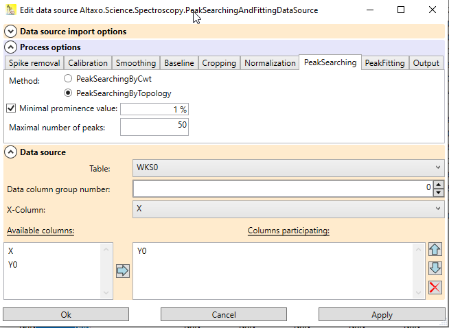
Fig. 1: Explanation of height and prominence value of the peak at x = 1500.

In Altaxo, only two options can be chosen:

• Minimal prominence: Designates the minimal prominence value of the peak. This is a relative value related to the y-span of the spectrum. The y-span of the spectrum is the difference of the highest intensity value and the lowest intensity value.

• Maximum number of peaks: Designates the maximum number of resulting peaks. If more peaks than this number are found, the peaks with the lowest prominence values are dropped, and only this number of peaks is included in the output.

Fig. 1: Options for 'Peak searching by topology'.

Peak searching by continuous wavelet transformation

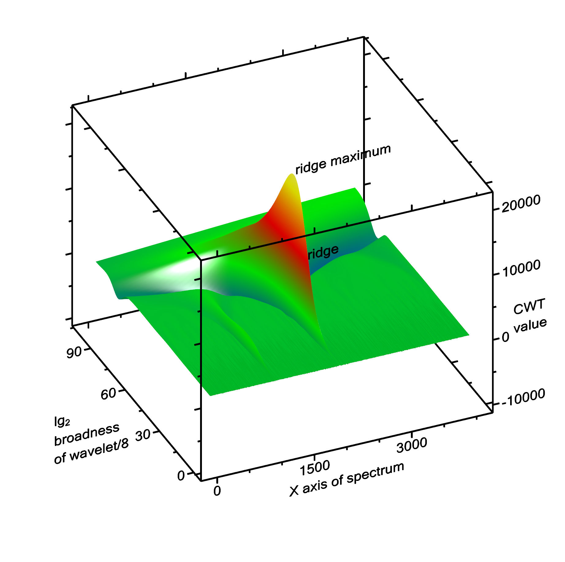
Peak searching by continuous wavelet transformation uses continuous wavelet transformation (CWT) to convolve the spectrum with a wavelet. In this case, the wavelet is a Ricker wavelet (also known as Mexican hat). Since the width of the peaks is not known at the beginning, the convolution has to be performed with the Ricker wavelet of different x-scales. The basic idea is, that the result of the convolution is maximal, if the width of the Ricker wavelet approximately corresponds with the width of the peak, and the center location of the wavelet and of the peak fall together. Around this maximum value, there is a mountain with very steep slopes in the "location" direction, but a ridge line in the "broadness of the wavelet" direction (Fig. 2).

The algorithm starts with a very narrow Ricker wavelet (which has a width of 1 point), and convolutes this with the signal. In each of the subsequent steps, the Ricker wavelet is made broader, and convoluted again with the signal. When the broadness of the wavelet exceeds the range of the entire spectrum, the algorithms stops. After this, ridge lines are detected. Each ridge line can correspond to a peak in the spectrum, but there are also some ridge lines that do not correspond to a peak. Therefore the ridge lines are filtered out using some criteria shown below.

Fig. 2: Example of a spectrum that is used for CWT transformation, see below.

Fig. 2: CWT transformation of the spectrum shown above. The ridge line and its maximum of the largest peak (at x = 2000) is labelled. To the left (at x = 1000) there is a second, much smaller ridge corresponding to the peak at x = 1000.

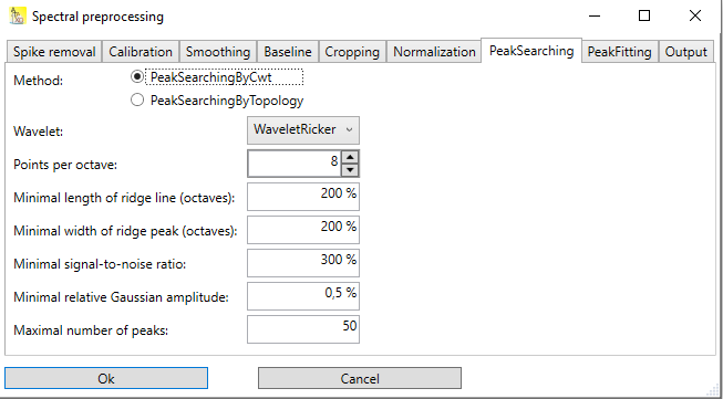
Fig. 3: Options for 'peaks searching by continuous wavelet transformation'.

The dialog contains various options, but most of them can be left at their default values:

• Wavelet: Choose between a Ricker wavelet, and a wavelet which is the 2nd derivative of the Ricker wavelet. The latter will enhance peaks located in shoulders of other peaks somewhat more.

• Points per octave: The default value 8 means the Ricker wavelet is made broader in steps of , i.e. after 8 steps the wavelet is twice as broad as before. The more points, the finer is the resolution of the determination of the peak width, but more steps require more evaluation time.

• Minimal length of ridge line. The minimal length of a ridge line that is required for the detection of a peak. The default value of 200% means that the ridge line must at least be 2 octaves long in order to be considered as a peak candidate.

• Minimal width of ridge peak (octaves). When following a ridge line, there is a maximum value, which is when the width of the wavelet is (roughly) equal to the width of the peak. The default value of 200% means that around that peak there should be no local maxima one octave higher and one octave lower. This will e.g. suppress local maxima on the ridge line caused by noise.

• Minimal signal-to-noise ratio: The value of the maximum on a ridge line must be considerably higher than the noise level in order to be the ridge line considered as a peak candidate. The default value of 300% means that the peak maximum must be 3 times higher than the noise level. Increasing this value will decrease the number of detected peaks, decreasing it will increase the number of detected peaks, but can cause to detect peaks, which are essentially noise.

• Minimal relative Gaussian amplitude: After a peak is detected and located, the amplitude of it (back in the signal domain) can be determined. The default value of 0.5% means that only those peaks are included in the result, that have a height which is at least 0.5% the y-span of the signal (difference of the signal maximum and the signal minimum values).

• Maximal number of peaks: Designates the maximum number of resulting peaks. If more peaks than this number are found, the peaks with the lowest height values are dropped, and only this number of peaks is included in the output.

References:

[1] Pan Du, Warren A. Kibbe, Simon M. Lin, "Improved peak detection in mass spectrum by incorporating continuous wavelet transform-based pattern matching", Bioinformatics Volume 22, Issue 17, August 2006 pp 2059–2065, https://doi.org/10.1093/bioinformatics/btl355

[2] Chao Yang, Zengyou He, Weichuan Yu, "Comparison of public peak detection algorithms for MALDI mass spectrometry data analysis", BMC Bioinformatics 10, 4 (2009), https://doi.org/10.1186/1471-2105-10-4

Peak fitting

After the peak searching step, the resulting approximate positions, widths, and heights of the peaks can be used as initial values for a subsequent peak fitting step.

Different fitting methods exists, which are described in the following.

Peak fitting by incremental peak addition

The method starts by searching the spectrum for the highest peak. Approximate position, width, and height of this peak is used as initial values for a fit function that contains only this peak and a baseline of user-defined polynomial order. The fit is executed. After fitting this peak, the fit function values are subtracted from the original spectrum (calculating the residual of the fit). In this residual, the highest peak is searched again. The position, width and height of the previous fit plus the approximate position, width, and height of the new peak is used as initial values for a fit function which has one more peak than the previous one. The fit is executed again. The process is repeated, adding more and more peaks, until a certain number of peaks are reached, or another stop criterion is fulfilled.

Note:
For the fitting method PeakFittingByIncrementalPeakAddition the peak searching step is not required. Please leave peak searching at the default value of topology search. Furthermore, baseline correction is also not required, since the fit function itself contains a polynomial baseline.

The options for this method are:

• Fit function: Choose the appropriate fit function.

• Order of baseline polynomial. Use a value of -1 for no baseline, a value of 0 for a constant baseline, 1 for a linear baseline. Values greater than 1 are possible too, but not recommended.

• Max. number of peaks: The maximum number of peaks that the fit function uses. The addition of peaks stops when this number is reached. Note that the final number of peaks can be less than this number, because after the fitting step, a pruning step follows, dropping the most insignificant peaks.

• Minimal relative height: The addition of peaks stops, if the highest peak in the residual has a height that is less the given factor times the original y-span of the spectrum (which is the difference of maximum y-value and minimum y-value of the spectrum).

• Minimal signal to noise: The addition of peaks stops, if the highest peak in the residual has a height that is less the given factor times the noise level.

• Minimal peak FWHM: If you know the resolution properties of your spectrometer, you can give here the minimal Full-Width-Half-Maximum value that a peak could reach. You can enter this value in points (checkbox cleared), or in the x-units of the spectrum (checkbox checked).

• Prune peaks factor: After the fitting, the most insignificant peaks can be dropped (i.e. not included in the result). This is done based on the Chi² value of the fit. The default value of 10% means, that peaks are dropped, as long as the new Chi² value of the fit remains below (100% + 10%) = 110% of the original Chi² value. Simply speaking, by dropping some peaks, the fit can go worse by 10%.

• Separate error evaluation with relative fit width: This choice only affects how the parameter errors (but not the parameter values itself) are calculated. For details see section "separate error evaluation for each peak".

Depending on the maximum number of peaks, and the complexity of the fit function, the evaluation can take considerable time, so please be patient! The advantage is, that by increasing the maximum number of peaks, you can model more and more details of your spectrum, leading to very precise fits.

Reference:

[1] Frank Alsmeyer, Wolfgang Marquardt, "Automatic generation of peak shaped models", Appl. Spectroscopy 58, 986-994 (2004), https://doi.org/10.1366/0003702041655421

Peak fitting separately

This method uses the result of the previous peak searching step. It assumed that each peak is well separated from the neighboring peaks, so that the peak reaches to the left and to the right (nearly) a value of zero.

Note:
The method assumes that the spectrum is baseline corrected, i.e. that the peak falls down to the left and to the right to a value of zero! Please use an appropriate baseline correction method.

The method fits each peak separately. If say the peak searching step results in 80 peaks, then 80 different fits are made, each with a fit function which contains only one peak.

This method has the following options:

• Fit function: Choose the appropriate fit function.

• Scale fit width by: Only the points in the spectrum in the vicinity of each peak are used for the fit. The default value of 200% means, that the approximate FWHM of the peak (as the result of the peak searching step) is multiplied with a factor of 2. The resulting width is then used for the fit range (i.e. 100% FWHM to the left and 100% FWHM to the right).

Peak fitting together (without or with separate variances)

In contrast to the method PeakFittingSeparately, this methods are better suited for peaks that can overlap.

Note:
The methods assume that the spectrum is baseline corrected, i.e. that if the peaks would not overlap, the peak would falls down to the left and to the right to a value of zero. Thus, the base of the peaks is assumed to be at zero. Please use an appropriate baseline correction method.

The method uses the resulting number of peaks from the peak searching step, and the approximate values for position, width, and height of the peaks, to create a fit function with that number of peaks and the initial values for position, width, and height. Then the fit is executed.

This methods have the following options:

• Fit function: Choose the appropriate fit function.

• Scale fit width by: Only the points in the spectrum in the vicinity of each peak are used for the fit. The default value of 200% means, that the approximate FWHM of the peak (as the result of the peak searching step) is multiplied with a factor of 2. The resulting width is then used for the fit range (i.e. 100% FWHM to the left and 100% FWHM to the right) around a peak. The fit ranges of all peaks are then combined into the final fit range.

The differences of the two methods are described in the next section.

Separate evaluation of parameter errors for each peak

If you are not interested in the resulting errors of the fit parameters, i.e. errors for position, width, height etc. of the peaks, you can skip this section.

The error of the fit parameters of a nonlinear fit is calculated from the Chi² value of the fit. Basically, it is defined as how much the parameter must be varied, so that the Chi² value becomes twice at high as before.

The problem here: when you make a fit that fits all peaks simultaneously (PeakFittingTogether and PeakFittingByIncrementalPeakAddition), then small peaks will not much contribute to the Chi² value. Which means, that the parameter of those small peaks must be varied unrealistically high in order to double the Chi² value of the fit.

In order to get more realistic error values for the parameters, not the global Chi² value of the fit is used, but the local Chi² value. To calculate the local Chi² value of a peak, only the points in the vicinity of that peak are used for summing up the squared differences between original spectrum and fit function. How many points are included depends on the value of the Scale fit width by value: the default value of 200% means that 200% of the FWHM of the peak (from the peak searching step) is used for calculating the local Chi² value of the peak. When the parameters of that peak are now varied, this local Chi² value is much more influenced (relative to the value before), than the global Chi² value, leading to more realistic results for the parameter errors.

These local Chi² values to calculate the parameter errors are utilized by PeakFittingTogetherWithSeparateVariances (otherwise equal to PeakFittingTogether), and for PeakFittingByIncrementalPeakAddition, if the checkbox Separate error eval. with relative fit width is checked.

Output

The output of the peak searching and peak fitting steps can be influenced by some options (see Fig. 1):

• Output preprocessed curve: if checked, the result of the preprocessing steps (everything except peak searching + fitting) is included in the resulting table.

• Output fit curve: The resulting fit curve is included in the resulting table. Since the fit curve looks better, if it has a higher resolution than the original spectrum, you can choose a sampling factor. A sampling factor of 1 means to include only the original x-values of the spectrum, a sampling factor of 3 adds to additional points between each pair of points of the original spectrum.

• Output separate peak curves: The resulting fit curve is included in the resulting table, but in contrast to the option described above, as separate peaks. In this way, it is easily to see from which peaks the fit curve is composed of. Here too, a sampling factor can be provided to enhance the resolution.

Note:
Checking Output fit curve, and Output separate peak curves not only include the data in the resulting table, but will also create a graph showing those curves together with the original spectrum. Later, when using this options in the data source of the resulting worksheet again, only the data are included, but the graph(s) will not be created again (of course they will show the changed data if they already exist).

Fig. 1: Dialog for the output options of the preprocessing / peak fitting pipeline.

Calibration of a Raman device with Neon light and a Silicon wafer

Objective

A Raman device consists of two, at first uncalibrated, parts:

• The spectrometer. The spectrometer pixels need to be attributed to their corresponding absolute wavelengths.

• The laser. The wavelength of the laser is approximately known, but it is necessary to determine the exact wavelength.

The objective of the calibration is to calibrate both the spectrometer and determine the absolute laser wavelength. With that information, the x-axis of all spectra measured subsequently could be adjusted to calibrated values.

What is needed

For that, two measurements are needed:

1. A measurement without laser (to exclude the influence of the laser wavelength). This measurement calibrates the spectrometer. Usually, the light of a small Neon lamp is directed into the Raman instrument, and a spectrum of the Neon light is taken. The position of the Neon bands is known, and with that information the wavelength of the spectrometer pixels can be calibrated.

2. A measurement with laser. In this measurement, a sample with a well defined peak, for which the Raman shift is known, is measured. Usually, a polished Silicon wafer is used for this measurement. In combination with the absolute wavelength calibration of the spectrometer with Neon light, the exact wavelength of the Laser light can be calculated.

Tips for measuring the Neon spectrum
Use exactly the same optical path that is used afterwards for measuring the Silicon. Block the laser light. Shine the light of a Neon lamp in your instrument and adjust exposure time to avoid both overexposure and underexposure. Then set the number of accumulations as high as possible to get a low noise level. A low noise level is important to get also the very small peaks close to the left and right sides of the spectrum, because everything outside the range of detected peaks needs to be extrapolated.

Tips for measuring the Silicon spectrum
Make sure the laser is switched on already for some time and now is stable. Adjust the exposure time to avoid both overexposure and underexposure. Set the number of accumulations as high as possible, but avoid too long measurement times because the Silicon is heating up (especially for 785 nm systems). Write down the room temperature (or ideally the temperature of the Silicon wafer). Measure the Silicon and the Neon spectra at the same day.

Data evaluation

Load both the Neon spectrum and the Silicon spectrum into an empty worksheet. For that, create an empty worksheet, and then use File → Import → Ascii, or File → Import → SPC or some of the other file import menu points, according to the file format of the spectra. Details on how to import can be find here.

Make sure that the x-axis of both spectra is marked as type "X". Take a look of the Neon spectrum by plotting it.

Neon calibration

Go back to the worksheet which contains both spectra, select the column with the Neon spectrum, and use the menu Analysis → Spectroscopy → Raman → Neon calibration. A dialog with many options opens, but for a first try, only two things are important:

• Chose the unit of the x-axis of the Neon spectrum you have loaded. In most cases, this would be the Raman shift in cm^-1.

• If the unit is indeed the Raman shift, the approximate wavelength of the laser is needed. Please enter it in the appropriate field (in nanometer). Typical wavelengths are 532 nm, 633 nm and 785 nm, but other systems exist as well.

Everything else could be left to default. Press OK to run the Neon calibration. A new worksheet is created, which should contain the calibration. Take a look at the Notes of this worksheet to check for errors during the execution of the calibration.

Typical errors are:

• The wrong column is selected as x-axis in the worksheet. For instance, many spectra (especially in .txt or .csv format) not only contain a column for the Raman shift, but also a column named Pixel number etc. Thus, maybe column Pixel number is selected as x-axis, but you think the x-axis is 'Raman shift'. You could check which column was used by opening the DataSource of the calibration table, and then check in Neon calibration data 1 (or Neon calibration data 2 if you are using the second Neon calibration), which x-column is currently used. The mistake of confusing Pixel number with Raman shift is really hard to detect, because on many systems both values are nearly in the same range!

• You have entered the wrong unit of the x-axis of the Neon spectrum. Some reasonability checks are made by the software, and if they fail, an error is reported.

• You have entered the wrong (approximate) wavelength of the laser. For instance, if you have a 785 nm system, but have forgotten to change the laser wavelength (which is by default 532 nm), the calibration will fail. This kind of error could not be detected by the software.

• The Neon spectrum is too noisy, so that too few peaks or too many peaks are detected. Try to adjust some options in the peak finding algorithm. You can use peak detection and finding (menu Analysis → Spectroscopy → PeakDetection & Finding) to search for appropriate settings, and then use those settings for calibration.

Silicon calibration

Next, do the silicon calibration. For this, go back to the worksheet containing the Silicon spectrum, select the column which contains the signal of the Silicon spectrum, and choose the menu point Analysis → Spectroscopy → Raman → Silicon calibration. The options can be left to their defaults, with two exceptions:

1. Enter the temperature of the room (or of the silicon wafer if it was measured)

2. Make sure that in the combobox "Calibration table" that calibration table is selected, which already contains the Neon calibration made before. If you only have one calibration in the entire Altaxo document, the combobox is already showing it, but if you have multiple calibrations, make sure that the right calibration table is selected.

Press OK. Now your calibration table should contain a full x-axis calibration. From now on you can use that calibration table in the preprocessing of spectra to adjust the x-axis to a calibrated x-axis.

Contents of the calibration table

If both the neon as well as the silicon calibration has been successfully performed, the calibration table consist of the following columns:

• NistNeonPeakWavelength [nm]
  Wavelength in nm of the neon peak tabulated in a table from NIST (National institute of Standards and Technology)

• MeasuredNeonPeakWavelength [nm]
  Wavelength in nm of the peak that was found in the neon spectrum used for calibration. Please note, that when the original x-axis of the neon spectrum was Raman shift (cm^-1), then the wavelength was calculated using the approximate laser wavelength that was provided in the neon calibration dialog.

• DifferenceOfPeakWavelengths [nm]
  Difference

• DifferenceOfPeakWavelengths.Err [nm]
  The error of the previous column, assuming that the NIST wavelength has a neglectable error. Thus, this column represents the errors of the fit position of the neon peaks.

• Neon1_PreprocessedUncalibrated_Wavelength [nm]
  X-axis values in nm of the neon spectrum. If the original x-axis of the neon spectrum was Raman shift (cm^-1), then the wavelength values in this column were calculated using the approximate laser wavelength that was provided in the neon calibration dialog.

• Neon1_PreprocessedCalibrated_Wavelength [nm]
  X-axis values in nm of the neon spectrum after the neon calibration. Thus, the values in this column represent absolute, calibrated wavelength values.

• Neon1_Preprocessed_Signal
  Y-values of the neon spectrum after execution of the preprocessing steps. These values can be plotted either using the uncalibrated wavelength x-axis, or the calibrated one (see the previous two columns).

• NeonCalibration_MeasuredWL [nm]
  X-axis values in nm of the neon spectrum. If the original x-axis of the neon spectrum was Raman shift (cm^-1), then the wavelength values in this column were calculated using the approximate laser wavelength that was provided in the neon calibration dialog.

• NeonCalibration_DifferenceWL [nm]
  Contains the difference wavelength values in nm. By adding these difference values to the uncalibrated x-axis values (see previous column), the calibrated x-axis in absolute nm is obtained.

• SiliconPeakShift [cm-1]
  This column only contains a single value, which is the peak position of the silicon peak (obtained from the fit of this peak).

• SiliconPeakShift.Err [cm-1]
  This column only contains a single value, which is the peak position error of the silicon peak (obtained from the fit of this peak).

• XCalibration_UncalibratedX
  Contains the uncalibrated x-axis in the unit in which the neon and silicon spectrum were provided.

• XCalibration_CalibratedX
  Contains the calibrated x-axis in the unit in which the neon and silicon spectrum were provided. The calibration uses here both the neon and silicon calibration.

• XCalibration_XDeviation
  Contains the difference between calibrated and uncalibrated x-axis values.

Note
Most of the columns in this table are for your information only. To apply an x-axis calibration to another spectrum, only the columns XCalibration_UncalibratedX and XCalibration_CalibratedX are necessary.

Intensity calibration of a Raman device with a known light source

Objective

The spectrometer of a Raman device has a sensitivity which is dependent on the wavelength. The sensitivity varies from device to device, even if they are coming from the same manufacturer.

The objective of the intensity calibration is to find a wavelength dependent correction function, which corrects the different sensitivities of the spectrometers. Although no absolute calibration is possible, this will make Raman spectra from different devices better comparable, because the relative heights of the peaks will be the same.

What is needed

For intensity calibration, a light source with a known spectrum is necessary:

• Either, a fluorescent glass is exited with the Raman laser, which will then emit light with a broad spectral distribution. Usually, for each laser wavelength, another glass is used. Such standards are available for instance from NIST, and they are accompanied by a description of the wavelength dependent intensity.

• Or, a known light source, for instance an LED with a known (preferable broad) spectrum, is used. The spectrum of the LED must cover the range of the spectrometer. Those light sources come with a certificate, in which the wavelength dependent intensity is described as a function.

What is measured

When using the fluorescent glass, follow the instructions accompanying this standard. The laser must be switched on for the measurement. Acquire a spectrum which is neither overexposed nor underexposed. Multiple accumulations can enhance the signal to noise ratio.

When using the known light source, the laser must not be switched on. Take a spectrum of the light source which is neither overexposed nor underexposed. Multiple accumulations can enhance the signal to noise ratio.

Important:
For both methods it is absolutely necessary to acquire a dark spectrum (a spectrum with laser and all other light sources off). On some instruments, a dark spectrum is acquired automatically, and is then part of the exported spectrum. Ideally, the exported spectrum contains already one column, in which the dark spectrum is subtracted from the signal spectrum.

Data evaluation

Load the acquired spectrum into an empty worksheet. For that, create an empty worksheet, and then use File → Import → Ascii, or File → Import → SPC or some of the other file import menu points, according to the file format of the spectra. Details on how to import can be find here.

Make sure that the x-axis of the spectrum is marked as type "X". Take a look at the spectrum by plotting it. It should have a broad distribution, i.e. the intensity should be high enough in all parts of the spectrum (except in the range close to the laser wavelength, where filter catch the light).

If the dark spectrum was exported to a separate file, then import that spectrum, too.

Intensity calibration

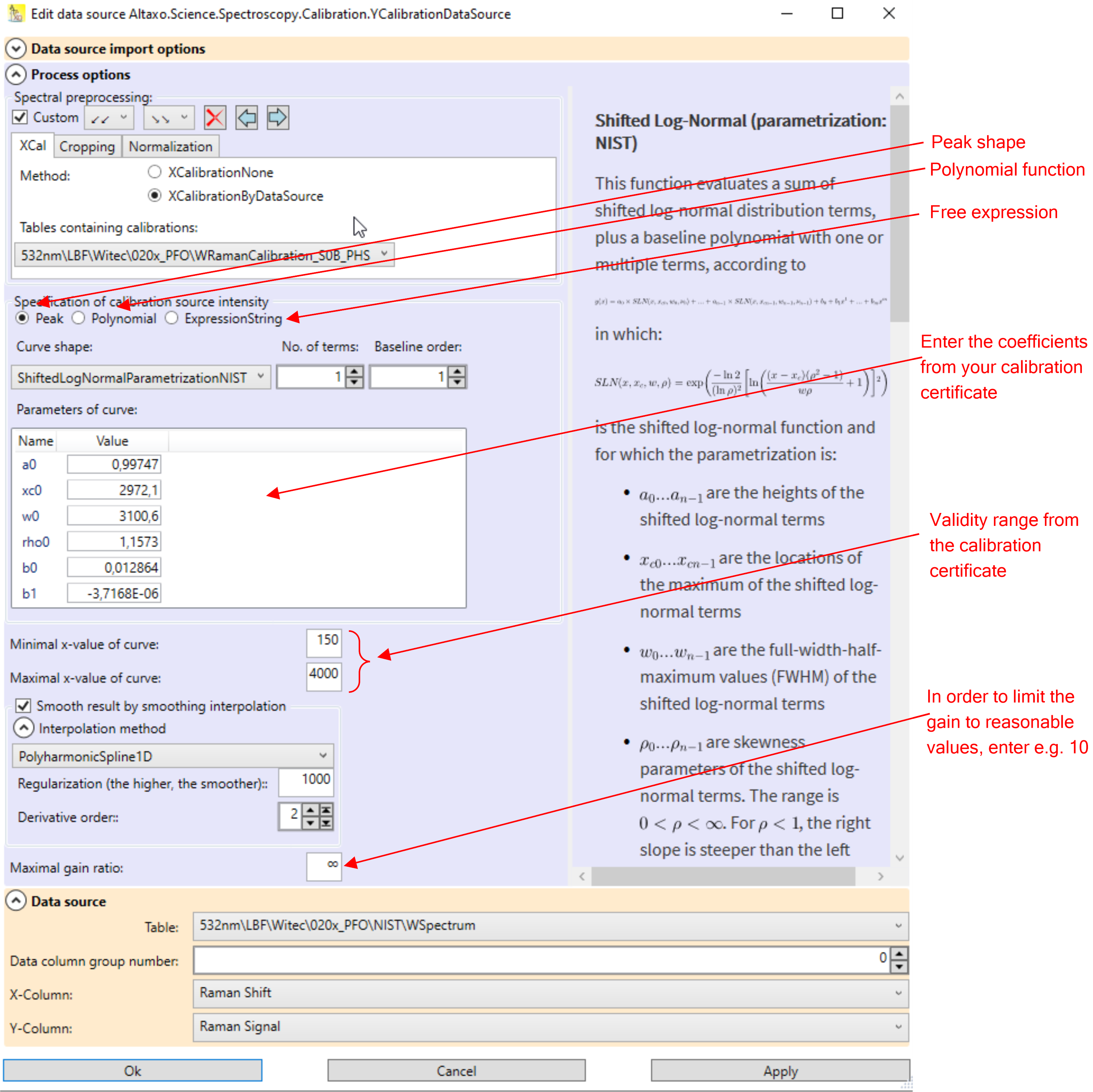
Go to the worksheet which contains the spectrum. If the worksheet contains a column in which the dark spectrum is already subtracted, then select this column. Otherwise, select the column with the y-values of the spectrum, and use the menu Analysis → Spectroscopy → Intensity calibration. A dialog opens.

Its upper part contain the spectral preprocessing pipeline. If the dark signal is already subtracted, no preprocessing should be used here. If it is not already subtracted, then use the tab 'Dark', choose SpectrumSubtraction, and provide the table which contains the dark spectrum and the x and y-column names of that spectrum.

In the lower part of the dialog, a function must be entered, which describes the intensity in dependence of the wavelength. Usually, a Gaussian distribution (with one term, with no baseline or a constant baseline is used). Make sure that the function you select is identical to the function that come with the certificate of the light source. The selected function is described in the right part of the dialog. Enter the parameters given on the certificate. Make also sure that the x-axis of your spectrum matches the x-axis unit given in the certificate. Example: if your x-axis is Raman shift, but on the certificate the x-axis unit is wavelength, then you can not perform intensity calibration.

Press OK to perform the intensity calibration. A new table is created, which contains the correction function.

Perform an intensity correction

In subsequent preprocessing operations, this calibration table can be used for intensity correction. Use the tab YCal of the preprocessing pipeline, select YCalibrationByDataSource, and in the combobox, choose the table containing the intensity calibration.

Next section: Appendix