Built-in fit functions |
Previous section: Appendix
This topic contains the following sections:
- Fit functions for chemistry
- Fit functions for sorption isotherms
- Diffusion fit functions
- General fit functions
- Kinetics related fit functions
- Materials related fit functions
- Fit functions for peaks (height parameter)
- Fit functions for probability density and peaks (area parameter)
- Relaxation fit functions
- Retardation fit functions
- Fit functions for transitions
- Fit functions for the viscosity versus the shear rate
MassBasedFloryDistribution
The molecular weight ![]() of a polymer which is synthesized in a reactor is often distributed according to a Flory distribution. The only parameter of this distribution (besides the area
of a polymer which is synthesized in a reactor is often distributed according to a Flory distribution. The only parameter of this distribution (besides the area ![]() ) is the ratio
) is the ratio ![]() of the probabilities of the termination step with respect to the chain prolongation step.
of the probabilities of the termination step with respect to the chain prolongation step.
This function evaluates a sum of mass based Flory distribution terms, plus a baseline polynomial with one or multiple terms, according to
in which:
 are the areas of the Flory terms (ATTENTION: only if integrated over the
  x-axis!)
 are the probability ratios of the termination reaction with respect to the chain prolongation reaction. The smaller this probability ratio, the longer the chains will become, i.e. the peak position is increased to higher molecular weight.
 are the coefficients of the baseline polynomial of order
 is the number of Flory distribution terms (
 )
)
- is the order of the baseline polynomial (set
 to disable the baseline polynomial)
 is the molecular weight of one monomer unit
The molecular weight of one monomer unit ![]() , the number of Flory distribution terms
, the number of Flory distribution terms ![]() and the order of the baseline polynomial
and the order of the baseline polynomial ![]() can be changed by double-clicking on the fit function. The default values are
can be changed by double-clicking on the fit function. The default values are ![]() ,
, ![]() and
and ![]() , corresponding to 1 term and no baseline.
, corresponding to 1 term and no baseline.
There is an additional property named IndependentVariableIsDecadicLogarithm. If this property is set to true, it is assumed that the x-axis is not the molecular weight, but the decadic logarithm of the molecular weight ![]() , which is often used in chemistry.
, which is often used in chemistry.
The domain of the function is ![]() (IndependentVariableIsDecadicLogarithm == false) or
(IndependentVariableIsDecadicLogarithm == false) or ![]() (IndependentVariableIsDecadicLogarithm == true).
(IndependentVariableIsDecadicLogarithm == true).
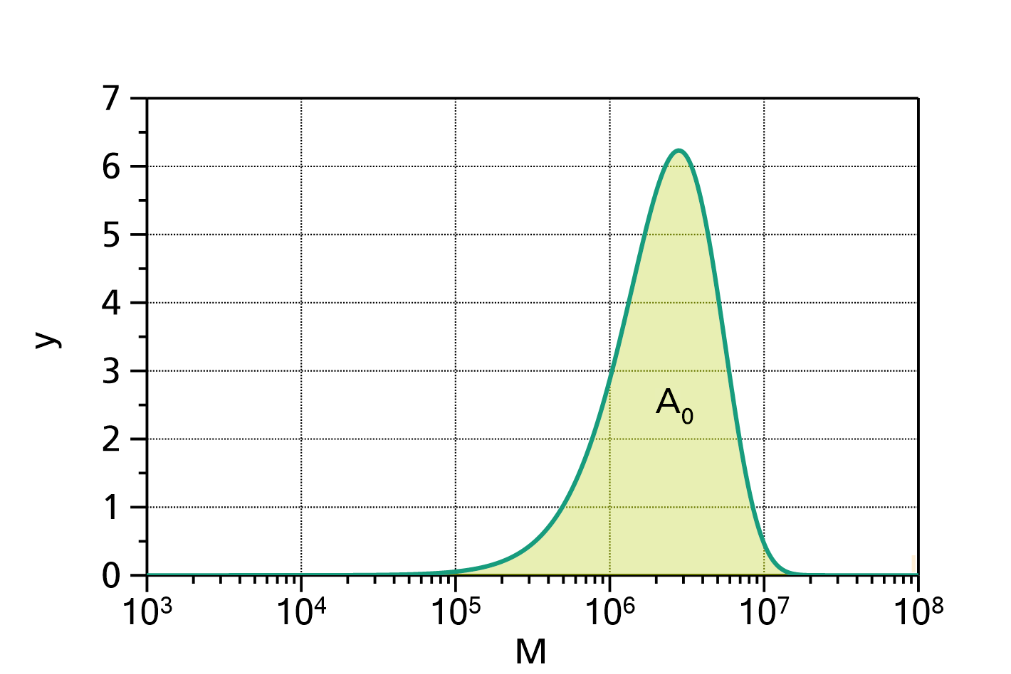
Fig. 1: MassBasedFloryDistribution (![]() ,
, ![]() ) with
) with ![]() and
and ![]() .
. ![]() was set to 14 (polyethylene).
was set to 14 (polyethylene).
References:
[1] Flory-Schulz distribution in Wikipedia
[2] João B. P. Soares, 'Polyolefin microstructural deconvolution methods: The good, the bad, and the ugly', https://doi.org/10.1002/cjce.24833
MassBasedFloryDistributionWithFixedGaussianBroadening
The molecular weight ![]() of a polymer which is synthesized in a reactor is often distributed according to a Flory distribution. The only parameter of this distribution (besides the area
of a polymer which is synthesized in a reactor is often distributed according to a Flory distribution. The only parameter of this distribution (besides the area ![]() ) is the ratio
) is the ratio ![]() of the probabilities of the termination step with respect to the chain prolongation step. The mass based Flory distribution can be described by:
of the probabilities of the termination step with respect to the chain prolongation step. The mass based Flory distribution can be described by:
Often, the measured signal in GPC is approximately broadened by a Gaussian distribution on the decadic logarithmic M (molecular weight) axis. This can be modelled by convoluting the Flory distribution with a Gaussian distribution on the (decadic) logarithmic M axis:

in which:
The broadness parameter ![]() is determined by calibration of the GPC column with reference substances. It is usually dependent on the molecular weight M of the peak.
is determined by calibration of the GPC column with reference substances. It is usually dependent on the molecular weight M of the peak.
The function MassBasedFloryDistributionWithFixedGaussianBroadening evaluates a sum of mass based, Gaussian broadened, Flory distribution terms, plus a baseline polynomial with one or multiple terms, according to
in which:

- are the areas of the Flory-Gauss terms (ATTENTION: only if integrated over the x-axis!)
- are the probability ratios of the termination reaction with respect to the chain prolongation reaction. The smaller this probability ratio, the longer the chains will become, i.e. the peak position is increased to higher molecular weight.
- are the coefficients of the baseline polynomial of order
The function
 is the dependence of the Gaussian broadening parameter
  on the molecular weight
  . This function is modeled as a polynomial of :
  . The polynomial coefficients of this function are fixed and are given in the settings of the fit function.
- is the number of Flory distribution terms ()
- is the order of the baseline polynomial (set to disable the baseline polynomial)
- is the molecular weight of one monomer unit
The molecular weight of one monomer unit ![]() , the number of Flory distribution terms
, the number of Flory distribution terms ![]() , the order of the baseline polynomial
, the order of the baseline polynomial ![]() , and the coefficients
, and the coefficients ![]() of the polynomial that models the
of the polynomial that models the ![]() dependency can be changed by double-clicking on the fit function. The default values are
dependency can be changed by double-clicking on the fit function. The default values are ![]() ,
, ![]() ,
, ![]() , and
, and ![]() corresponding to 1 term, no baseline, and no broadening.
corresponding to 1 term, no baseline, and no broadening.
There is an additional property named IndependentVariableIsDecadicLogarithm. If this property is set to true, it is assumed that the x-axis is not the molecular weight, but the decadic logarithm of the molecular weight ![]() , which is often used in chemistry. An additional property which can be set is the accuracy of the evaluation, since the function can not be evaluated analytically.
, which is often used in chemistry. An additional property which can be set is the accuracy of the evaluation, since the function can not be evaluated analytically.
The domain of the function is ![]() (IndependentVariableIsDecadicLogarithm == false) or
(IndependentVariableIsDecadicLogarithm == false) or ![]() (IndependentVariableIsDecadicLogarithm == true).
(IndependentVariableIsDecadicLogarithm == true).
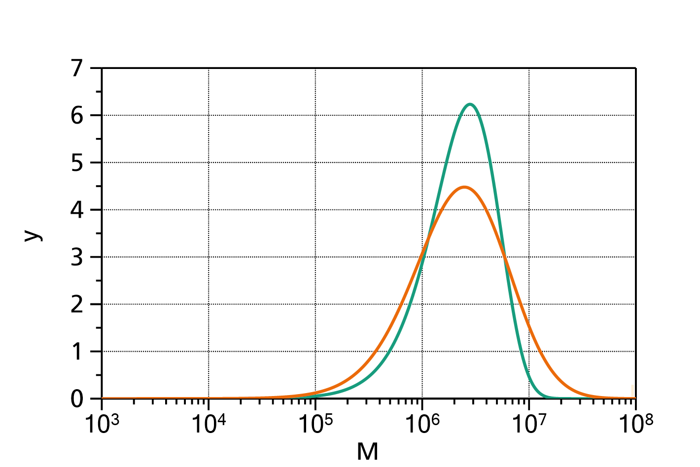
Fig. 1: Comparison of a MassBasedFloryDistribution without Gaussian broadening (green) and with Gaussian broadening (orange). The parameters are ![]() ,
, ![]() ,
, ![]() and
and ![]() . For the broadened function, the broadening setting was
. For the broadened function, the broadening setting was ![]() .
. ![]() was set to 14 (polyethylene).
was set to 14 (polyethylene).
References:
[1] Flory-Schulz distribution in Wikipedia
[2] João B. P. Soares, 'Polyolefin microstructural deconvolution methods: The good, the bad, and the ugly', https://doi.org/10.1002/cjce.24833
Mass uptake according to the Brunauer-Emmett-Teller model (BET model)
The mass uptake of e.g. water by a sample material in dependence of the water activity can be described by the following formula:
in which:
 is the sample mass in dependence on the water activity
 is the water activity (0 ... 1) (approx. the relative humidity in percent / 100)
 is sample mass at activity x=0 (dry conditions)
 is the monolayer moisture content
 is a constant (usually much greater than 1)
The domain of the function is ![]() .
.
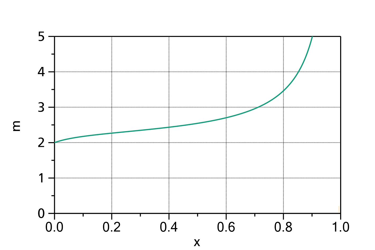
Fig. 1: Brunauer-Emmett-Teller model with ![]() ,
, ![]() and
and ![]() .
.
References:
[1] S. Brunauer, P.H. Emmett, E. Teller, "Adsorption of Gases in Multimolecular Layers", J. Am. Chem. Soc. 60 (1938), 2, pp. 309–319, DOI: 10.1021/ja01269a023
Mass uptake according to the Guggenheim-Anderson-de Boer model (GAB model)
The mass uptake of e.g. water by a sample material in dependence of the water activity can be described by the following formula:
in which:
- is the sample mass in dependence on the water activity
- is the water activity (0 ... 1) (approx. the relative humidity in percent / 100)
- is sample mass at activity x=0 (dry conditions)
- is the monolayer moisture content
- is a constant (usually much greater than 1)
 is another constant (usually close to 1). If
  , this model is identical to the Brunauer-Emmett-Teller model.
The domain of the function is ![]() if
if ![]() .
.
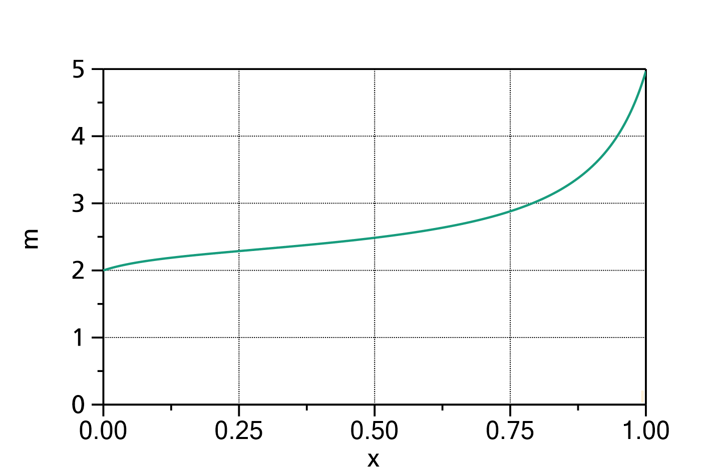
Fig. 1: Guggenheim-Anderson-de Boer function with ![]() ,
, ![]() ,
, ![]() and
and ![]() .
.
References:
[1] R.B. Anderson, "Modification of the Brunauer, Emmett and Teller equation", Journal of the American Chemical Society, 68 (1946), pp. 686–691, DOI: 10.1021/ja01208a049
[2] R.B. Anderson, W.K. Hall, "Modification of the Brunauer, Emmett and Teller equation II.", Journal of the American Chemical Society, 70 (1948), pp. 1727–1734, DOI: doi.org/10.1021/ja01185a017
[3] C. van den Berg, S. Bruin, "Water activity and its estimation in food systems: Theoretical aspects", in L. B. Rockland & G. F. Stewart (Eds.), Water Activity: Influences on Food Quality (pp. 1–61). Academic Press 1981, doi: 10.1016/b978-0-12-591350-8.50007-3
[4] R. Andrade, R. Lemus M., C.E.Perez, "Models of sorption isotherms for food: uses and limitations", Vitae, Revista de la Facultad de Quimica Farmaceutica, 18 (2011), pp. 325-334, ISSN 0121-4004
Mass uptake according to the Guggenheim-Anderson-de Boer model (GAB model) in simplified parametrization
The mass uptake of e.g. water by a sample material in dependence of the water activity can be described with the following formula:
in which:
- is the sample mass in dependence on the water activity
- is the water activity (0 ... 1) (relative humidity in percent / 100)
- is mass at x=0 (dry conditions)
 ,
,  , and
, and  are (empirical) parameter
The domain of the function is ![]() .
.
The relation of the simplified parameters (![]() ) to the original parameters (
) to the original parameters (![]() ) of the GAB model are:
) of the GAB model are:
or
respectively.
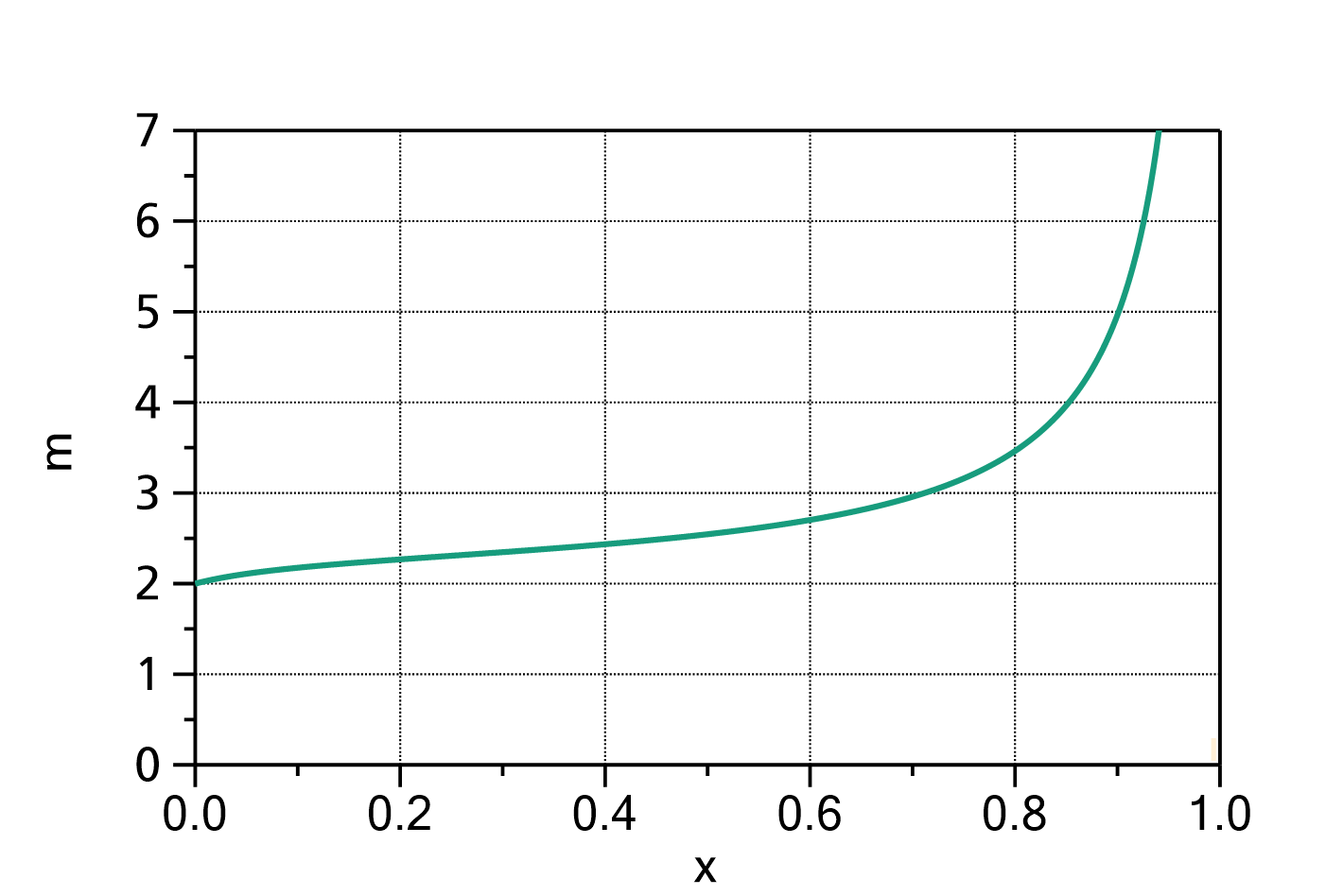
Fig. 1: Guggenheim-Anderson-de Boer model (simplified parametrization) with ![]() ,
, ![]() ,
, ![]() and
and ![]() .
.
References:
[1] R.B. Anderson, "Modification of the Brunauer, Emmett and Teller equation", Journal of the American Chemical Society, 68 (1946), pp. 686–691, DOI: 10.1021/ja01208a049
[2] R.B. Anderson, W.K. Hall, "Modification of the Brunauer, Emmett and Teller equation II.", Journal of the American Chemical Society, 70 (1948), pp. 1727–1734, DOI: 10.1021/ja01185a017
[3] C. van den Berg, S. Bruin, "Water activity and its estimation in food systems: Theoretical aspects", in L. B. Rockland & G. F. Stewart (Eds.), Water Activity: Influences on Food Quality (pp. 1–61). Academic Press 1981, DOI: 10.1016/b978-0-12-591350-8.50007-3
[4] R. Andrade, R. Lemus M., C.E. Perez, "Models of sorption isotherms for food: uses and limitations", Vitae, Revista de la Facultad de Quimica Farmaceutica, 18 (2011), pp. 325-334, ISSN 0121-4004
Mass uptake according to the Halsey model
The mass uptake of e.g. water by a sample material in dependence of the water activity can be described by the following formula:
in which:
- is the relative mass uptake (if
 ) or the sample mass in dependence on the water activity
- is the water activity (0 ... 1) (approx. the relative humidity in percent / 100)
- is sample mass at activity x=0 (dry conditions)
- is a constant (usually much greater than 1)
- is an exponent
The domain of the function is ![]() .
.
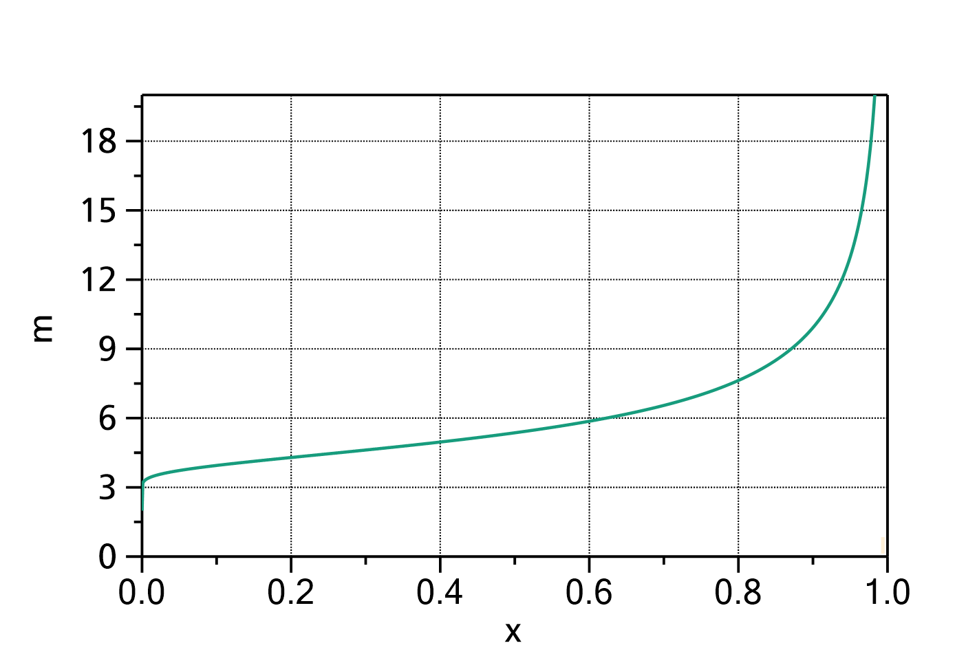
Fig. 1: Halsey model with ![]() ,
, ![]() and
and ![]() .
.
References:
[1] R. Andrade, R. Lemus M., C.E.Perez, "Models of sorption isotherms for food: uses and limitations", Vitae, Revista de la Facultad de Quimica Farmaceutica, 18 (2011), pp. 325-334, ISSN 0121-4004
Mass uptake according to the Henderson model
The mass uptake of e.g. water by a sample material in dependence of the water activity can be described by the following formula:
in which:
- is the relative mass uptake (if ) or the sample mass in dependence on the water activity
- is the water activity (0 ... 1) (approx. the relative humidity in percent / 100)
- is sample mass at activity x=0 (dry conditions)
- is a constant (usually much greater than 1)
- is an exponent
The domain of the function is ![]() .
.
Fig. 1: Henderson model with ![]() ,
, ![]() and
and ![]() .
.
References:
[1] R. Andrade, R. Lemus M., C.E.Perez, "Models of sorption isotherms for food: uses and limitations", Vitae, Revista de la Facultad de Quimica Farmaceutica, 18 (2011), pp. 325-334, ISSN 0121-4004
Mass uptake according to the Iglesias-Chirife model
The mass uptake of e.g. water by a sample material in dependence of the water activity can be described by the following formula:
which results in:
in which:
- is the relative mass uptake (if ) or the sample mass in dependence on the water activity
- is the water activity (0 ... 1) (approx. the relative humidity in percent / 100)
- is a sample mass offset
 are constants
 is the relative mass uptake at
  (? this is questionable, it doesn't result from the equation ?)
The domain of the function is ![]() .
.
Fig. 1: Iglesias-Chirife model with ![]() ,
, ![]() ,
, ![]() and
and ![]() .
.
References:
[1] Iglesias, H.A.; Chirife, J. "An Empirical Equation for Fitting Water Sorption Isotherms of Fruits and Related Products", Canadian Institute of Food Science and Technology Journal, 11(1) 1978, 12-15. doi: 10.1016/S0315-5463(78)73153-6
[2] R. Andrade, R. Lemus M., C.E.Perez, "Models of sorption isotherms for food: uses and limitations", Vitae, Revista de la Facultad de Quimica Farmaceutica, 18 (2011), pp. 325-334, ISSN 0121-4004
Mass uptake according to the Langmuir model
The mass uptake of e.g. water by a sample material in dependence of the water activity can be described by the following formula:
in which:
- is the relative mass uptake (if ) or the sample mass in dependence on the water activity
- is the water activity (0 ... 1) (approx. the relative humidity in percent / 100)
- is sample mass at activity x=0 (dry conditions)
- is the monolayer mass uptake
- is a constant (usually much greater than 1)
The domain of the function is ![]() .
.
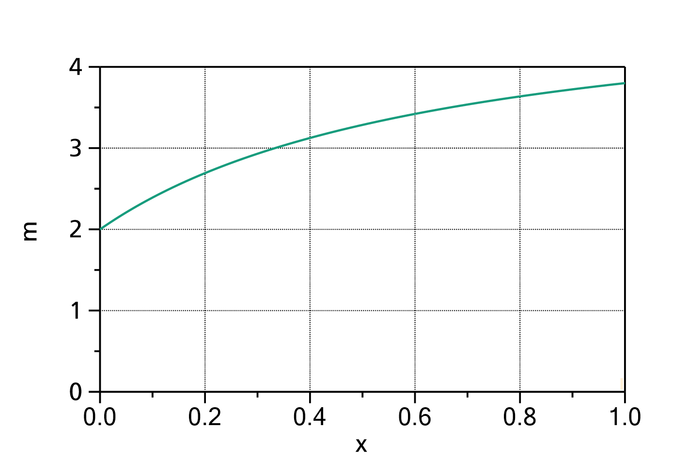
Fig. 1: Langmuir model with ![]() ,
, ![]() and
and ![]() .
.
References:
[1] R. Andrade, R. Lemus M., C.E.Perez, "Models of sorption isotherms for food: uses and limitations", Vitae, Revista de la Facultad de Quimica Farmaceutica, 18 (2011), pp. 325-334, ISSN 0121-4004
Mass uptake according to the Oswin model
The mass uptake of e.g. water by a sample material in dependence of the water activity can be described by the following formula:
in which:
- is the relative mass uptake (if ) or the sample mass in dependence on the water activity
- is the water activity (0 ... 1) (approx. the relative humidity in percent / 100)
- is sample mass at activity x=0 (dry conditions)
- is a constant (usually much greater than 1)
- is an exponent
The domain of the function is ![]() .
.
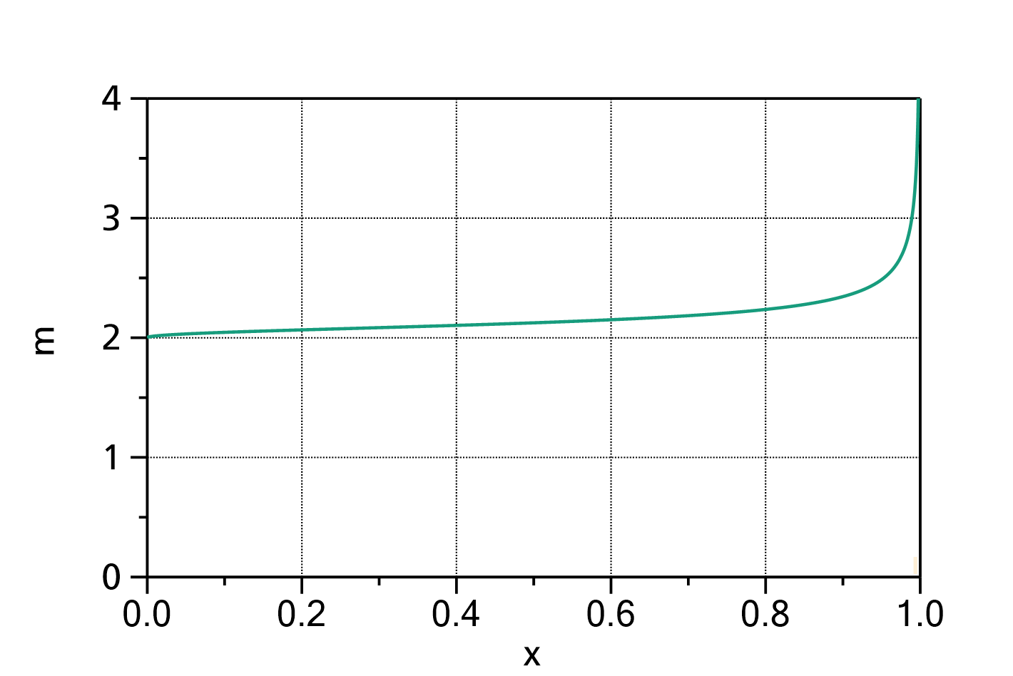
Fig. 1: Oswin model with ![]() ,
, ![]() and
and ![]() .
.
References:
[1] R. Andrade, R. Lemus M., C.E.Perez, "Models of sorption isotherms for food: uses and limitations", Vitae, Revista de la Facultad de Quimica Farmaceutica, 18 (2011), pp. 325-334, ISSN 0121-4004
Mass uptake according to the Peleg model
The mass uptake of e.g. water by a sample material in dependence of the water activity can be described by the following formula:
in which:
- is the relative mass uptake (if ) or the sample mass in dependence on the water activity
- is the water activity (0 ... 1) (approx. the relative humidity in percent / 100)
- is sample mass at activity x=0 (dry conditions)
 are factors
 are exponents (usually one exponent is chosen to be less than one, the other greater than 1)
The domain of the function is ![]() .
.
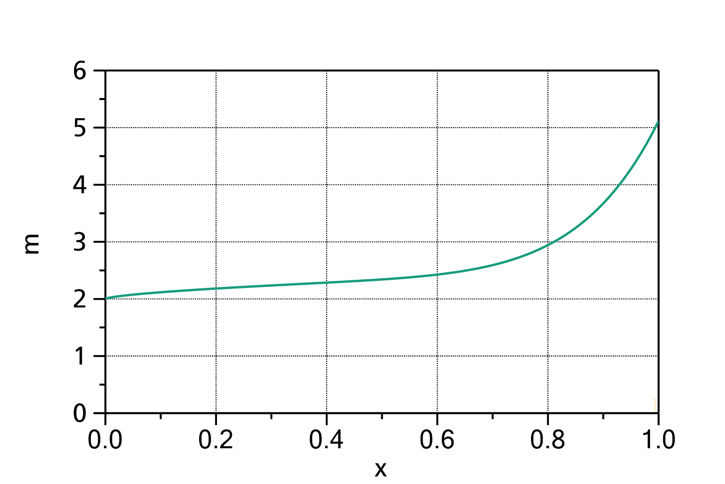
Fig. 1: Peleg model with ![]() ,
, ![]() ,
, ![]() ,
, ![]() and
and ![]() .
.
References:
[1] R. Andrade, R. Lemus M., C.E.Perez, "Models of sorption isotherms for food: uses and limitations", Vitae, Revista de la Facultad de Quimica Farmaceutica, 18 (2011), pp. 325-334, ISSN 0121-4004
Mass uptake according to the Smith model
The mass uptake of e.g. water by a sample material in dependence of the water activity can be described by the following formula:
in which:
- is the relative mass uptake (if ) or the sample mass in dependence on the water activity
- is the water activity (0 ... 1) (approx. the relative humidity in percent / 100)
- is sample mass at activity x=0 (dry conditions)
- is a constant (usually much greater than 1)
The domain of the function is ![]() .
.
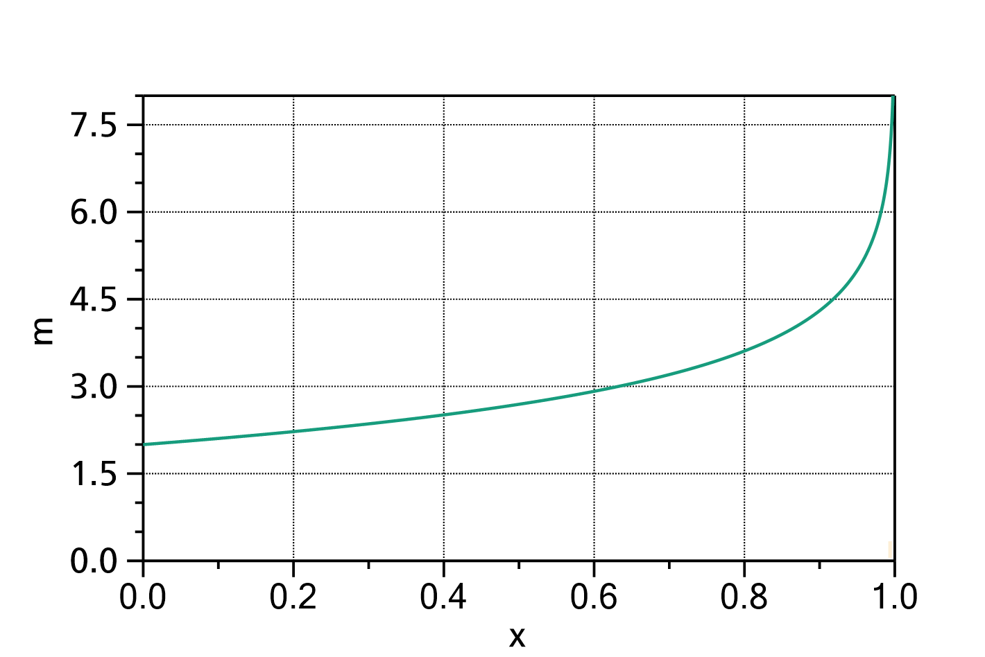
Fig. 1: Smith model with ![]() and
and ![]() .
.
References:
[1] S.E. Smith, “Sorption of water vapor by proteins at high polymers” J. Am. Chem. Soc., vol. 69, 1947, pp, 646–651, doi: 10.1021/ja01195a053
[2] R. Andrade, R. Lemus M., C.E.Perez, "Models of sorption isotherms for food: uses and limitations", Vitae, Revista de la Facultad de Quimica Farmaceutica, 18 (2011), pp. 325-334, ISSN 0121-4004
Mass change of a cylinder after a concentration step
This function evaluates the mass change of a cylinder with radius ![]() after a step of the outer concentration in dependence of the time
after a step of the outer concentration in dependence of the time ![]() . The length of the cylinder is considered infinite, i.e. diffusion from the end faces of the cylinder is neglected.
. The length of the cylinder is considered infinite, i.e. diffusion from the end faces of the cylinder is neglected.
in which:
 is the dimensionless reduced variable:
  ,
, 
 is the nth zero point of the Bessel function
 is the time (independent variable)
 is the time where the concentration step occurs, i.e. the beginning of the diffusion process (parameter)
 is the diffusion coefficient (parameter)
- is the mass of the plane sheet before the concentration step, i.e. for
 (parameter)
 is the mass change due to the concentration step (parameter)
 is the radius of the cylinder (property of the fit function)
The radius of the cylinder ![]() can be changed by double-clicking on the fit function. The default value is
can be changed by double-clicking on the fit function. The default value is ![]() .
.
The domain of the independent variable ![]() is
is ![]() .
.
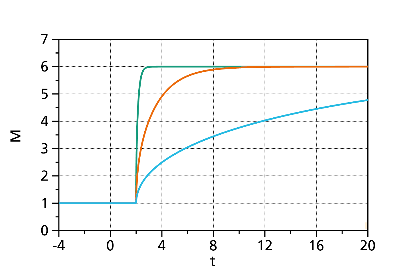
Fig. 1: Mass change of a cylinder after a concentration step with ![]() ,
, ![]() ,
, ![]() ,
, ![]() and
and ![]() (green curve),
(green curve), ![]() (orange curve), and
(orange curve), and ![]() (cyan curve).
(cyan curve).
Ref. [1 ]: Crank, "The Mathematics of Diffusion", 2nd edition, 1975, Oxford University Press, p. 73
Mass change of a cylinder after an exponential equilibration concentration change
This function evaluates the mass change of a cylinder with the radius ![]() after an exponential equilibration concentration change of the outer concentration in dependence of the time
after an exponential equilibration concentration change of the outer concentration in dependence of the time ![]() , i.e. the concentration varies with a characteristic time constant
, i.e. the concentration varies with a characteristic time constant ![]() according to:
according to:
The length of the cylinder is considered infinite, i.e. diffusion from the end faces of the cylinder is neglected. The mass ![]() is then:
is then:
in which:
- is the dimensionless reduced variable: ,
 is the dimensionless reduced time constant:
- is the nth zero point of the Bessel function
- is the time (independent variable)
- is the time where the concentration change starts, i.e. the beginning of the diffusion process (parameter)
- is the diffusion coefficient (parameter)
- is the mass of the plane sheet before the concentration step, i.e. for (parameter)
- is the mass change due to the concentration step (parameter)
 is the characteristic time constant of the concentration change
- is the radius of the cylinder (property of the fit function)
The radius of the cylinder ![]() can be changed by double-clicking on the fit function. The default value is
can be changed by double-clicking on the fit function. The default value is ![]() .
.
The domain of the independent variable ![]() is
is ![]() .
.
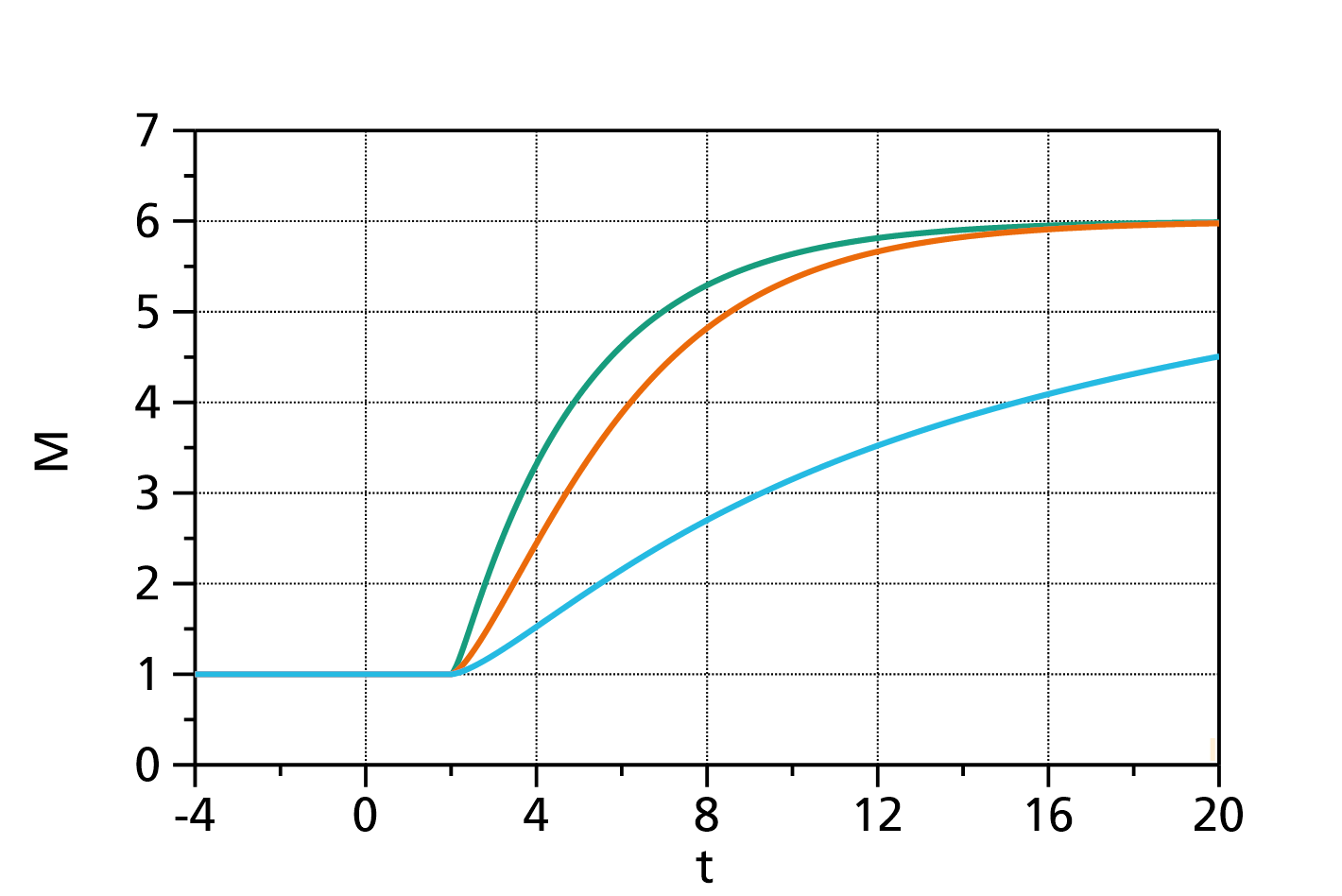
Fig. 1: Mass change of a cylinder after an exponential concentration change with ![]() ,
, ![]() ,
, ![]() ,
, ![]() ,
, ![]() and
and ![]() (green curve),
(green curve), ![]() (orange curve), and
(orange curve), and ![]() (cyan curve).
(cyan curve).
Ref. [1 ]: Crank, "The Mathematics of Diffusion", 2nd edition, 1975, Oxford University Press, p. 75
Mass change of a plane sheet after a concentration step
This function evaluates the mass change of a plane sheet of the total thickness ![]() after a step of the outer concentration in dependence of the time
after a step of the outer concentration in dependence of the time ![]() . The diffusion takes place from both sides of the plane sheet. The lateral dimensions of the sheet are considered infinite, i.e. diffusion from the edges of the sheet is neglected.
. The diffusion takes place from both sides of the plane sheet. The lateral dimensions of the sheet are considered infinite, i.e. diffusion from the edges of the sheet is neglected.
in which:
- is the dimensionless reduced variable:
 ,
, - is the time (independent variable)
- is the time where the concentration step occurs, i.e. the beginning of the diffusion process (parameter)
- is the diffusion coefficient (parameter)
- is the mass of the plane sheet before the concentration step, i.e. for (parameter)
- is the mass change due to the concentration step (parameter)
 is the thickness of the plane sheet (property of the fit function)
The thickness of the plane sheet ![]() can be changed by double-clicking on the fit function. The default value is
can be changed by double-clicking on the fit function. The default value is ![]() .
.
The domain of the independent variable ![]() is
is ![]() .
.
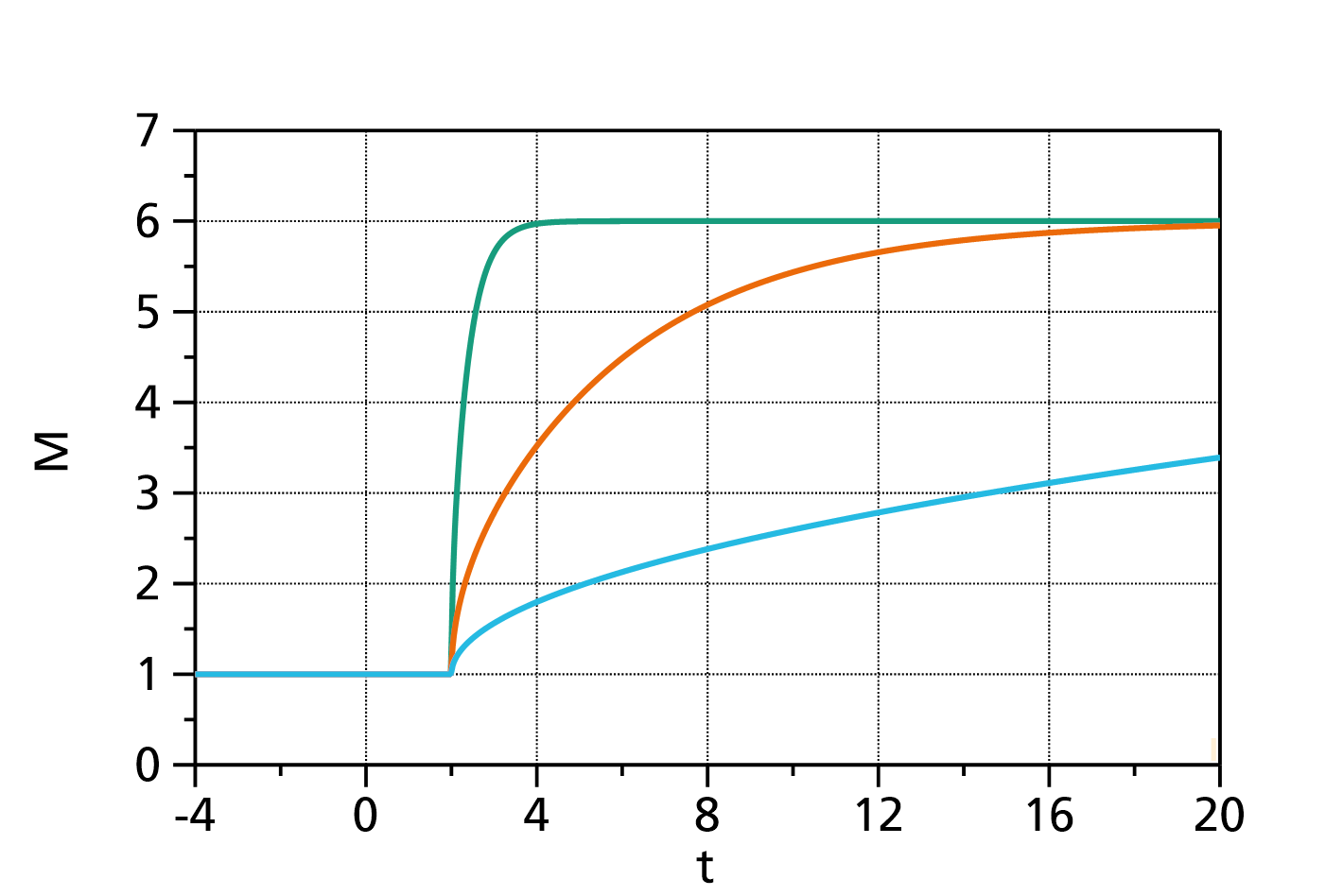
Fig. 1: Mass change of a plane sheet after a concentration step with ![]() ,
, ![]() ,
, ![]() ,
, ![]() and
and ![]() (green curve),
(green curve), ![]() (orange curve), and
(orange curve), and ![]() (cyan curve).
(cyan curve).
Ref. [1 ]: Crank, "The Mathematics of Diffusion", 2nd edition, 1975, Oxford University Press, p. 48
Mass change of a plane sheet after an exponential equilibration concentration change
This function evaluates the mass change of a plane sheet of the total thickness ![]() after an exponential equilibration concentration change of the outer concentration in dependence of the time
after an exponential equilibration concentration change of the outer concentration in dependence of the time ![]() , i.e. the concentration varies with a characteristic time constant
, i.e. the concentration varies with a characteristic time constant ![]() according to:
according to:
The diffusion takes place from both sides of the plane sheet. The lateral dimensions of the sheet are considered infinite, i.e. diffusion from the edges of the sheet is neglected. The mass ![]() is then:
is then:
in which:
- is the dimensionless reduced variable: ,
- is the dimensionless reduced time constant:

- is the time (independent variable)
- is the time where the concentration change starts, i.e. the beginning of the diffusion process (parameter)
- is the diffusion coefficient (parameter)
- is the mass of the plane sheet before the concentration step, i.e. for (parameter)
- is the mass change due to the concentration step (parameter)
- is the characteristic time constant of the concentration change
- is the thickness of the plane sheet (property of the fit function)
The thickness of the plane sheet ![]() can be changed by double-clicking on the fit function. The default value is
can be changed by double-clicking on the fit function. The default value is ![]() .
.
The domain of the independent variable ![]() is
is ![]() .
.
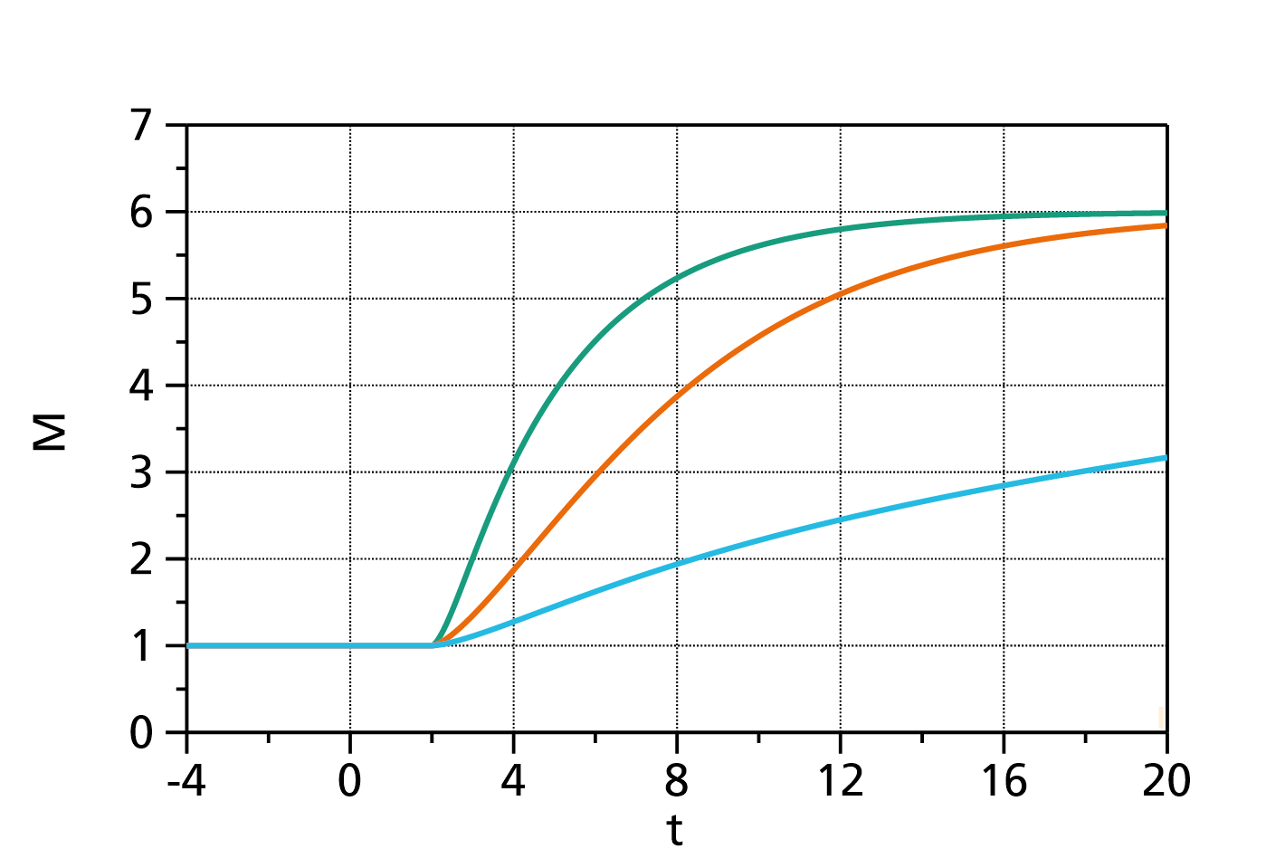
Fig. 1: Mass change of a plane sheet after an exponential concentration change with ![]() ,
, ![]() ,
, ![]() ,
, ![]() ,
, ![]() and
and ![]() (green curve),
(green curve), ![]() (orange curve), and
(orange curve), and ![]() (cyan curve).
(cyan curve).
Ref. [1 ]: Crank, "The Mathematics of Diffusion", 2nd edition, 1975, Oxford University Press, p. 53
Mass change of a sphere after a concentration step
This function evaluates the mass change of a sphere of radius ![]() after a step of the outer concentration in dependence of the time
after a step of the outer concentration in dependence of the time ![]() .
.
in which:
- is the dimensionless reduced variable: ,
- is the time (independent variable)
- is the time where the concentration step occurs, i.e. the beginning of the diffusion process (parameter)
- is the diffusion coefficient (parameter)
- is the mass of the plane sheet before the concentration step, i.e. for (parameter)
- is the mass change due to the concentration step (parameter)
- is the radius of the sphere (property of the fit function)
The radius of the sphere ![]() can be changed by double-clicking on the fit function. The default value is
can be changed by double-clicking on the fit function. The default value is ![]() .
.
The domain of the independent variable ![]() is
is ![]() .
.
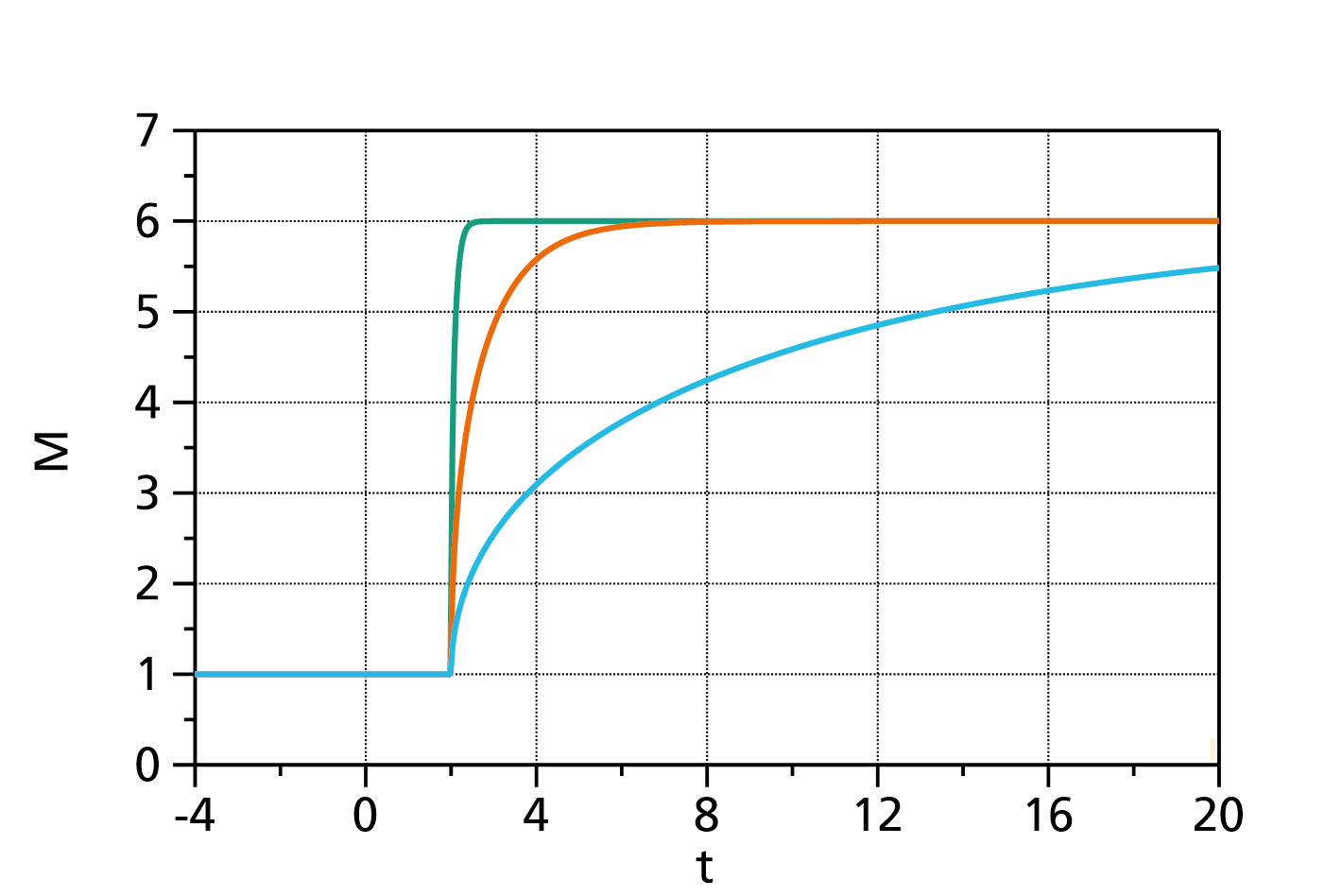
Fig. 1: Mass change of a sphere after a concentration step with ![]() ,
, ![]() ,
, ![]() ,
, ![]() and
and ![]() (green curve),
(green curve), ![]() (orange curve), and
(orange curve), and ![]() (cyan curve).
(cyan curve).
Ref. [1 ]: Crank, "The Mathematics of Diffusion", 2nd edition, 1975, Oxford University Press, p. 91
Mass change of a sphere after an exponential equilibration concentration change
This function evaluates the mass change of a sphere with the radius ![]() after an exponential equilibration concentration change of the outer concentration in dependence of the time
after an exponential equilibration concentration change of the outer concentration in dependence of the time ![]() , i.e. the concentration varies with a characteristic time constant
, i.e. the concentration varies with a characteristic time constant ![]() according to:
according to:
The mass ![]() is then:
is then:
in which:
- is the dimensionless reduced variable: ,
- is the dimensionless reduced time constant:
- is the nth zero point of the Bessel function
- is the time (independent variable)
- is the time where the concentration change starts, i.e. the beginning of the diffusion process (parameter)
- is the diffusion coefficient (parameter)
- is the mass of the plane sheet before the concentration step, i.e. for (parameter)
- is the mass change due to the concentration step (parameter)
- is the characteristic time constant of the concentration change
- is the radius of the sphere (property of the fit function)
The radius of the sphere ![]() can be changed by double-clicking on the fit function. The default value is
can be changed by double-clicking on the fit function. The default value is ![]() .
.
The domain of the independent variable ![]() is
is ![]() .
.
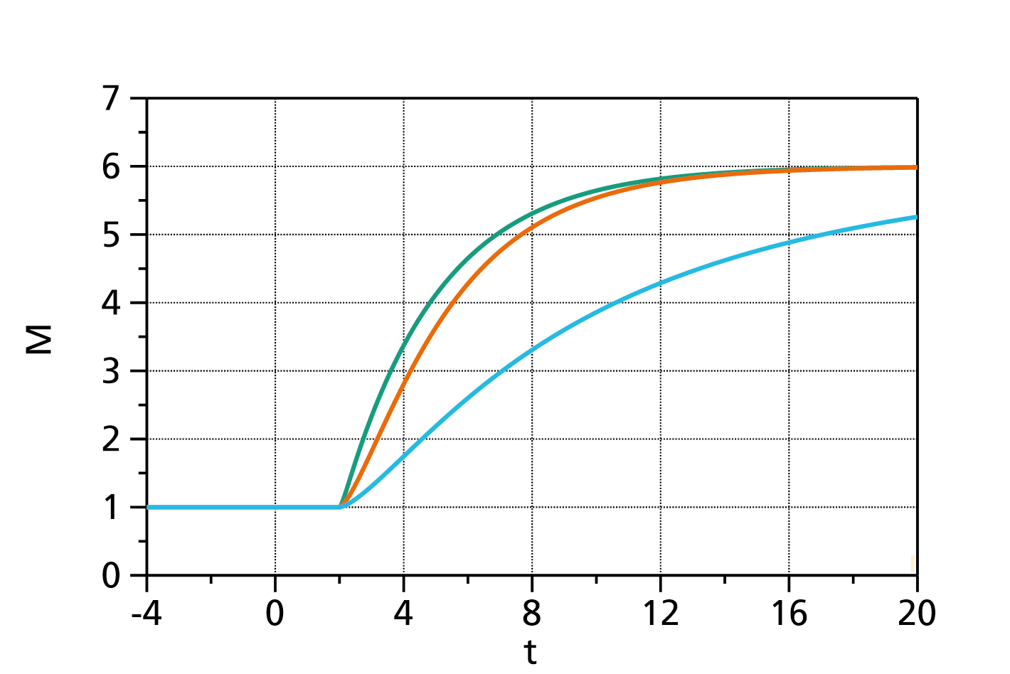
Fig. 1: Mass change of a sphere after an exponential concentration change with ![]() ,
, ![]() ,
, ![]() ,
, ![]() ,
, ![]() and
and ![]() (green curve),
(green curve), ![]() (orange curve), and
(orange curve), and ![]() (cyan curve).
(cyan curve).
Ref. [1 ]: Crank, "The Mathematics of Diffusion", 2nd edition, 1975, Oxford University Press, p. 92
ExponentialDecay
This function evaluates an exponential decay with one or multiple terms according to
in which:
 is the value of the base line (value of y for
  )
)
- ..
 are the prefactors of the exponential decay terms
 ...
...  are the characteristic times
- is the number of exponential terms
The number of terms ![]() can be changed by double-clicking on the fit function. The default value is
can be changed by double-clicking on the fit function. The default value is ![]() .
.
The domain of the function is ![]() .
.
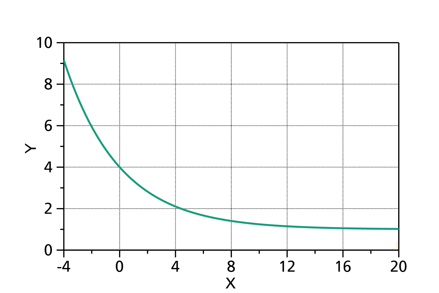
Fig. 1: Exponential decay with ![]() ,
, ![]() , and
, and ![]() .
.
ExponentialEquilibration
This function evaluates an exponential equilibration process with one or multiple terms according to

in which:
- is the starting value (and the value for
 )
)
 is the starting point of the equilibration process
- .. are the prefactors of the exponential equilibration terms
- ... are the characteristic times
- is the number of exponential terms
The number of terms ![]() can be changed by double-clicking on the fit function. The default value is
can be changed by double-clicking on the fit function. The default value is ![]() .
.
The domain of the function is ![]() .
.
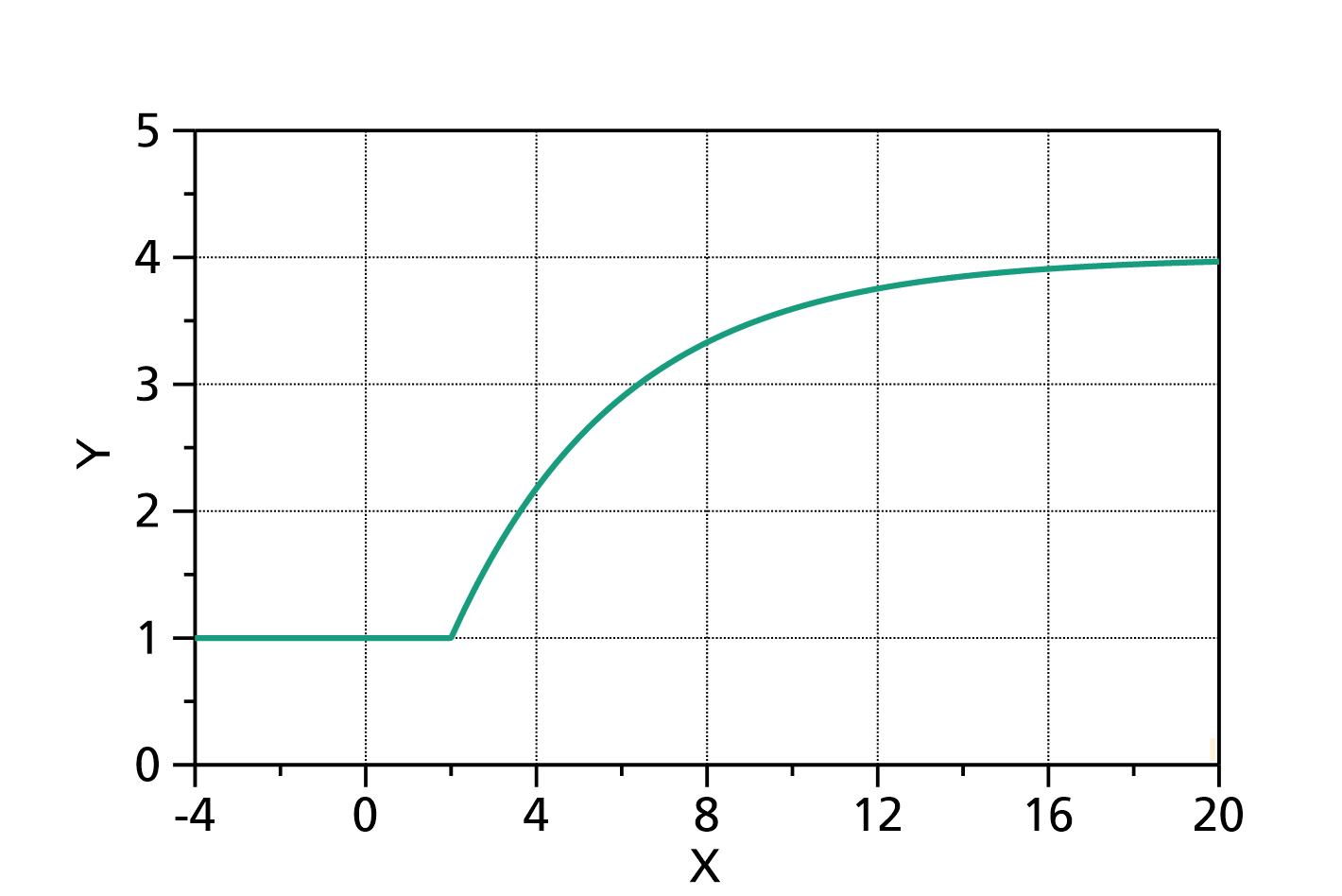
Fig. 1: Exponential equilibration with ![]() ,
, ![]() ,
, ![]() and
and ![]() .
.
Exponential growth
This function evaluates an exponential growth with one or multiple terms according to
in which:
- is the value of the base line (value of y for
 )
)
- .. are the prefactors of the exponential terms
- ... are the characteristic times
- is the number of exponential terms
The number of terms ![]() can be changed by double-clicking on the fit function. The default value is
can be changed by double-clicking on the fit function. The default value is ![]() .
.
The domain of the function is ![]() .
.
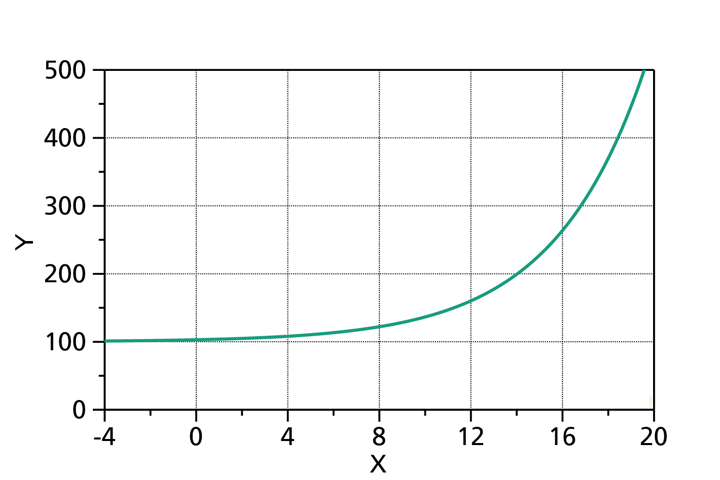
Fig. 1: Exponential growth with ![]() ,
, ![]() and
and ![]() .
.
Polynomial
This function evaluates an polynomial with one or multiple terms, and both positive and negative exponents, according to
in which:
 are the polynomial coefficients for positive exponents
 ...
...  are the polynomial coefficients for negative exponents
- is the order of the polynom for positive exponents
- is the order of the polynom for negative exponents
The polynomial orders ![]() and
and ![]() can be changed by double-clicking on the fit function. The default value is
can be changed by double-clicking on the fit function. The default value is ![]() and
and ![]() . If some of the terms are not needed, set their corresponding coefficients fixed to zero.
. If some of the terms are not needed, set their corresponding coefficients fixed to zero.
The domain of the function is ![]() . If
. If ![]() ,
, ![]() is excluded.
is excluded.
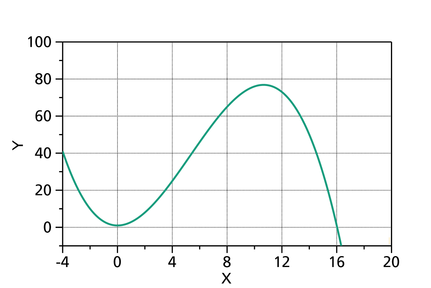
Fig. 1: Polynomial (![]() ,
, ![]() ) with
) with ![]() ,
, ![]() ,
, ![]() and
and ![]() .
.
Power law (with pre-factors)
This function evaluates a power law with one or multiple terms according to
in which:
- is the value of the base line (value of y for
 )
)
- .. are the pre-factors of the terms
 ...
...  are the exponents
- is the number of terms
The number of terms ![]() can be changed by double-clicking on the fit function. The default value is
can be changed by double-clicking on the fit function. The default value is ![]() . Strictly speaking, the function is a power law only if
. Strictly speaking, the function is a power law only if ![]() and
and ![]() .
.
The domain of the function is ![]() if all
if all ![]() are positive, or
are positive, or ![]() if some of the exponents are negative.
if some of the exponents are negative.
Note:
Even if you set the exponents fixed to integer values, the domain of the function is not extended to the full range! If the full range is neccessary, try to use Polynomial instead.
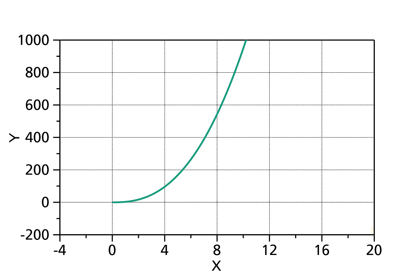
Fig. 1: Power law with ![]() ,
, ![]() and
and ![]() with linear x- and y-axes.
with linear x- and y-axes.
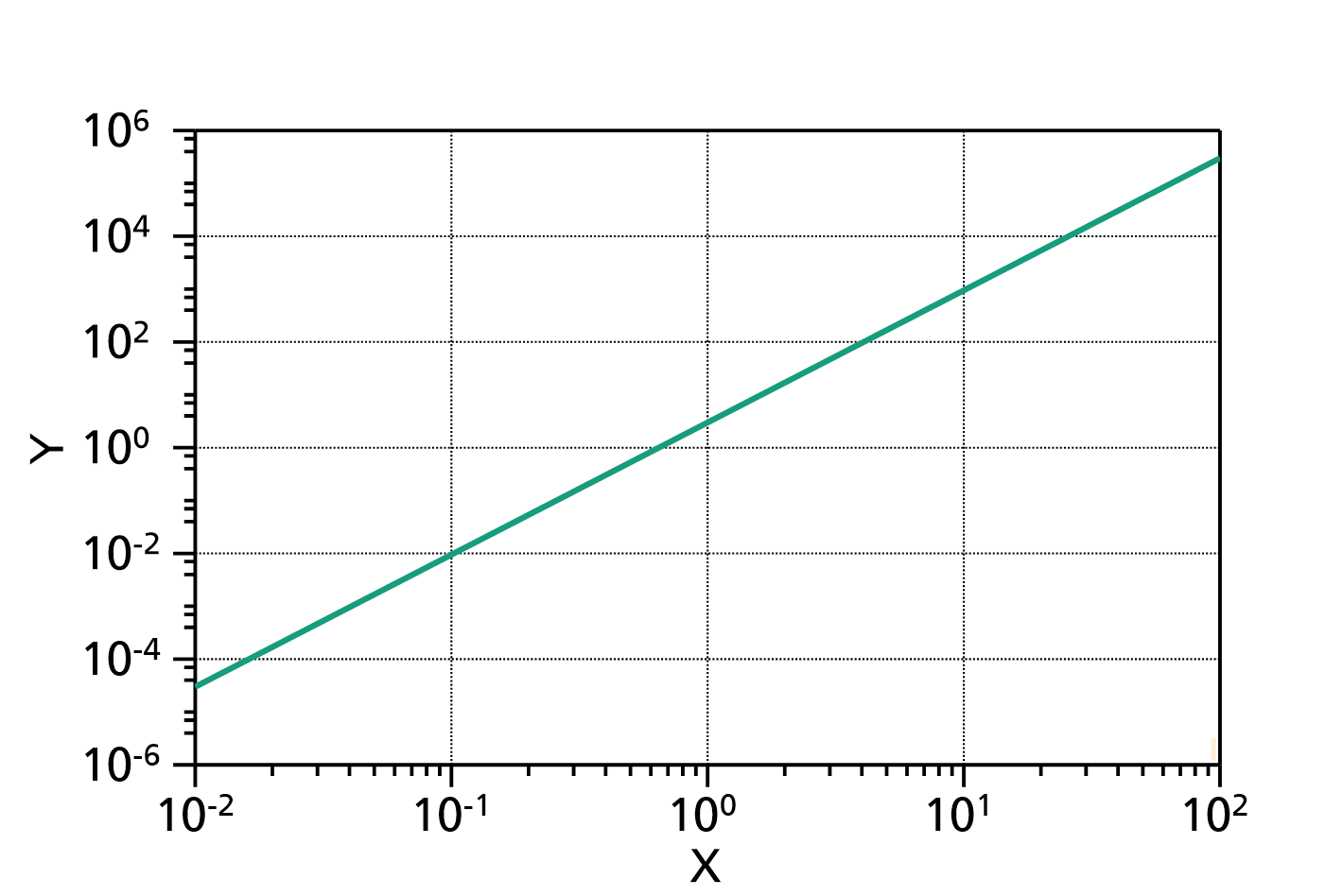
Fig. 2: Power law with the same parameters ![]() ,
, ![]() and
and ![]() in a double-logarithmic plot.
in a double-logarithmic plot.
Power law (with ratios)
This function evaluates a power law with one or multiple terms according to
in which:
- is the value of the base line (value of y for )
- .. are the denominators of the terms
- ... are the exponents
- is the number of terms
The number of terms ![]() can be changed by double-clicking on the fit function. The default value is
can be changed by double-clicking on the fit function. The default value is ![]() . Strictly speaking, the function is a power law only if
. Strictly speaking, the function is a power law only if ![]() and
and ![]() .
.
The domain of the function is ![]() if all
if all ![]() and all
and all ![]() are positive,
are positive, ![]() if all
if all ![]() are positive and all
are positive and all ![]() are negative, and, if some of the exponents are negative, the value
are negative, and, if some of the exponents are negative, the value ![]() is not included.
is not included.
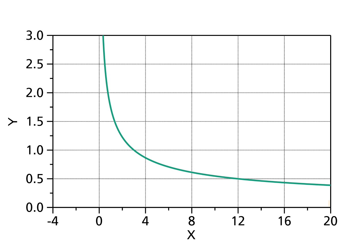
Fig. 1: Power law (ratio) with ![]() ,
, ![]() and
and ![]() with linear x- and y-axes.
with linear x- and y-axes.
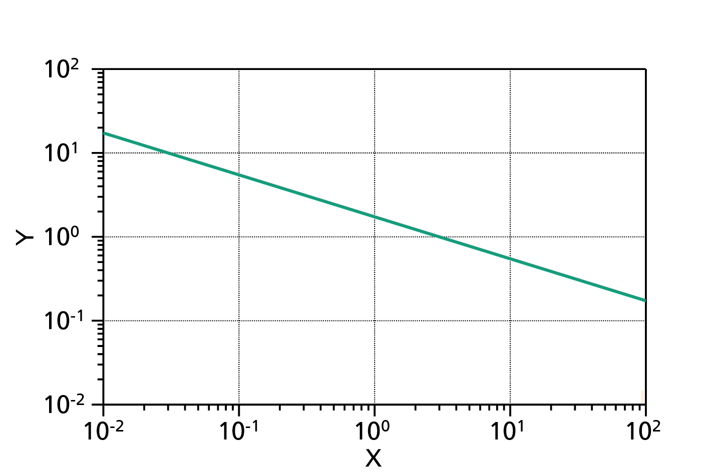
Fig. 2: Power law (ratio) with the same parameters ![]() ,
, ![]() and
and ![]() in a double-logarithmic plot.
in a double-logarithmic plot.
Rational
This function evaluates a rational polynom with one or multiple terms in the nominator and in the denominator according to
in which:
- ..
 are the coefficients of the nominator polynom
- .. are the coefficients of the denominator polynom
- is the polynomial order of the nominator polynom
- is the polynomial order of the denominator polynom
In order to avoid covariance between the 0th order coefficients ![]() and
and ![]() , in this formula
, in this formula ![]() is set to
is set to ![]() . Please use RationalInverse if a free value of
. Please use RationalInverse if a free value of ![]() is preferred.
is preferred.
The polynomial orders ![]() and
and ![]() can be changed by double-clicking on the fit function. The default value is
can be changed by double-clicking on the fit function. The default value is ![]() and
and ![]() .
.
The domain of the function is ![]() , with some points (poles) excluded, at which the denominator becomes zero.
, with some points (poles) excluded, at which the denominator becomes zero.
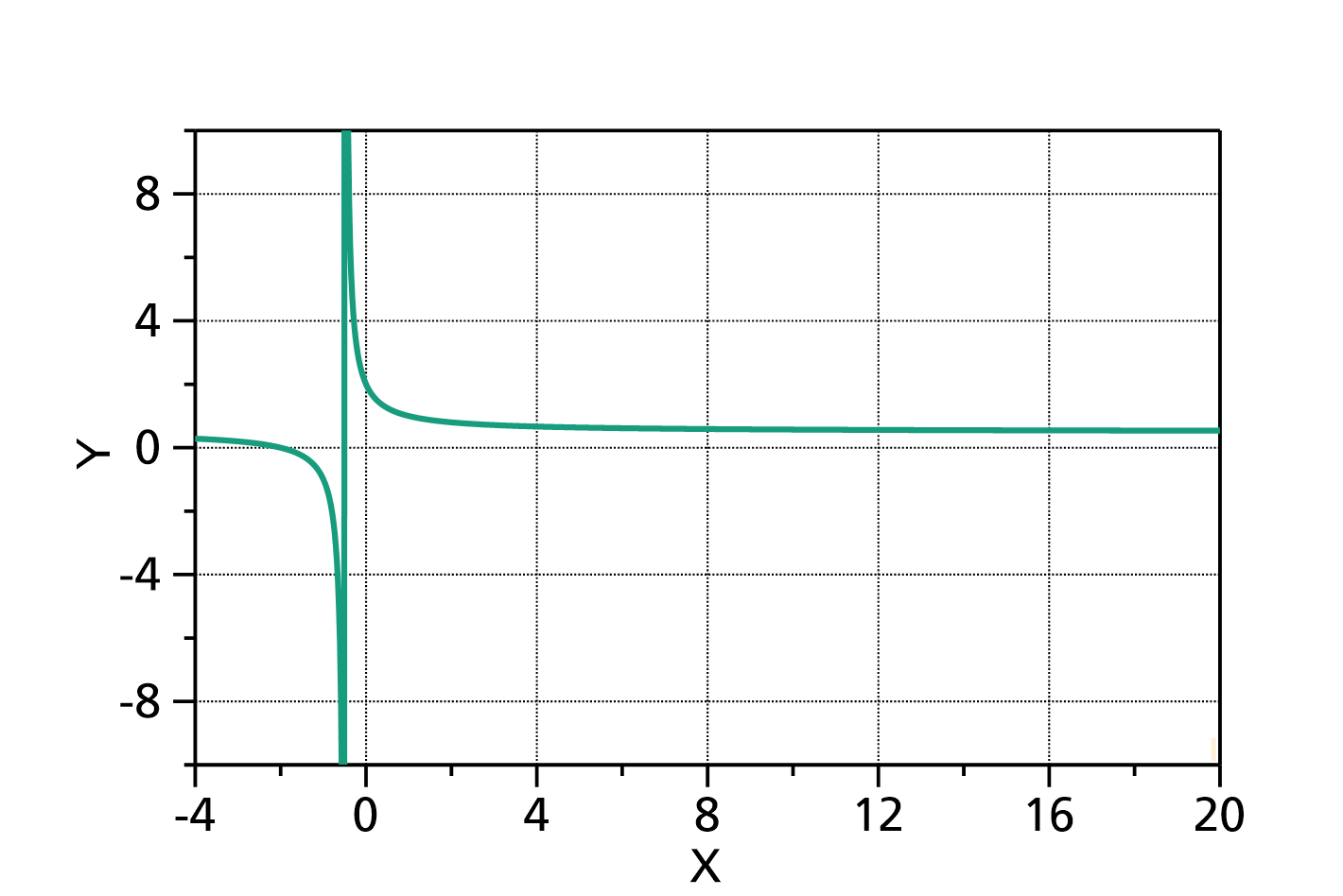
Fig. 1: Rational ![]() , i.e. with
, i.e. with ![]() ,
, ![]() ,
, ![]() and
and ![]() .
.
RationalInverse
This function evaluates a rational polynom with one or multiple terms in the nominator and in the denominator according to
in which:
- .. are the coefficients of the nominator polynom
 .. are the coefficients of the denominator polynom
- is the polynomial order of the nominator polynom
- is the polynomial order of the denominator polynom
In order to avoid covariance between the 0th order coefficients ![]() and
and ![]() , in this formula
, in this formula ![]() is set to
is set to ![]() . Please use Rational if a free value of
. Please use Rational if a free value of ![]() is preferred.
is preferred.
The polynomial orders ![]() and
and ![]() can be changed by double-clicking on the fit function. The default value is
can be changed by double-clicking on the fit function. The default value is ![]() and
and ![]() .
.
The domain of the function is ![]() , with some points (poles) excluded, at which the denominator becomes zero.
, with some points (poles) excluded, at which the denominator becomes zero.
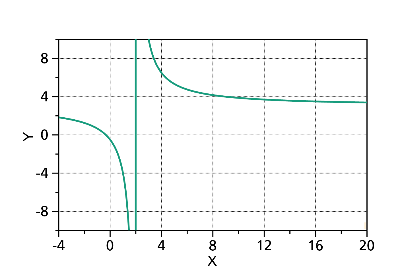
Fig. 1: RationalInverse ![]() , i.e. with
, i.e. with ![]() ,
, ![]() ,
, ![]() and
and ![]() .
.
Stretched exponential decay
(also known as Kohlrausch decay)
This function evaluates a stretched exponential decay process starting at ![]() with one or multiple terms according to
with one or multiple terms according to

in which:
- is the starting point of the decay process. If this value is known, you should enter the value and set this parameter to fixed.
- is the value for
- .. are the pre-factors of the exponential terms
- ... are the characteristic times
 ...
...  are the exponents, usually in the range
- is the number of exponential terms
The number of terms ![]() can be changed by double-clicking on the fit function. The default value is
can be changed by double-clicking on the fit function. The default value is ![]() .
.
The domain of the function is ![]() . The function values are set to constant for
. The function values are set to constant for ![]() .
.
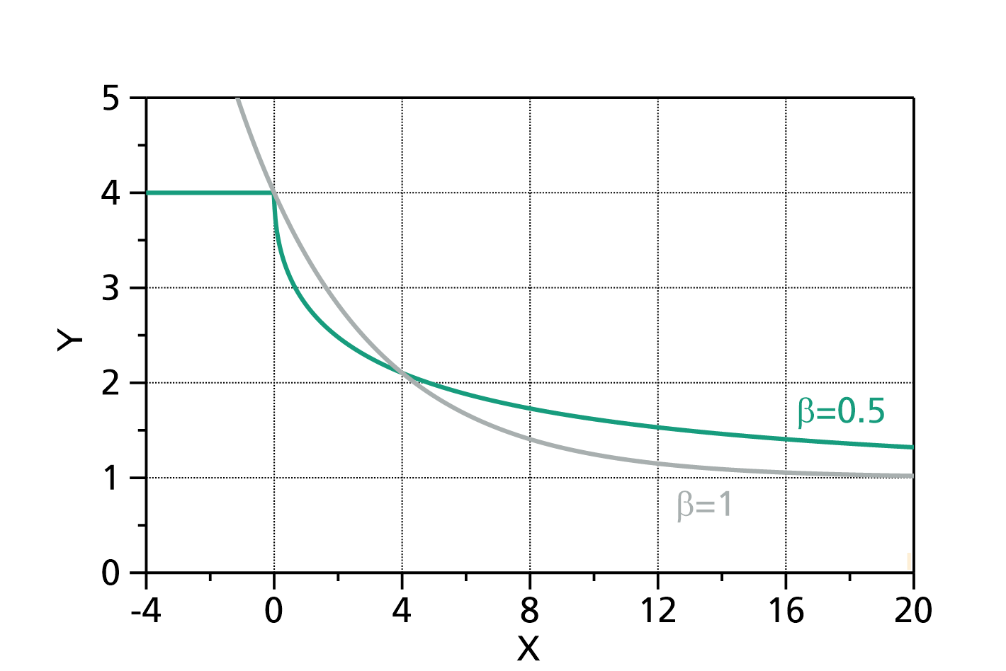
Fig. 1: Stretched exponential decay with ![]() ,
, ![]() ,
, ![]() ,
, ![]() , and
, and ![]() (green) in comparison to a 'normal' exponential decay function with the same parameters (grey). Note that the 'normal' exponential decay has varying function values both for
(green) in comparison to a 'normal' exponential decay function with the same parameters (grey). Note that the 'normal' exponential decay has varying function values both for ![]() and
and ![]() , whereas the stretched exponential decay is constant for
, whereas the stretched exponential decay is constant for ![]() .
.
Stretched exponential equilibration
This function evaluates a stretched exponential equilibration process with one or multiple terms according to

in which:
- is the starting point of the equilibration process. If this value is known, you should enter the value and set this parameter to fixed.
- is the starting value (and the value for )
- .. are the pre-factors of the exponential equilibration terms
- ... are the characteristic times
- ... are the exponents, usually in the range
- is the number of exponential terms
The number of terms ![]() can be changed by double-clicking on the fit function. The default value is
can be changed by double-clicking on the fit function. The default value is ![]() .
.
The domain of the function is ![]() .
.
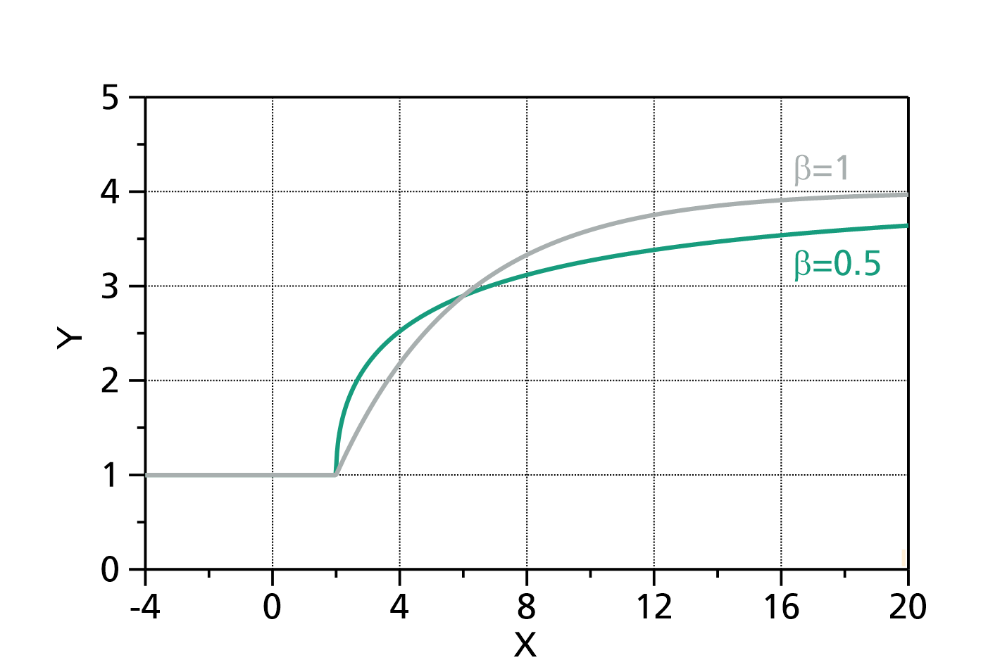
Fig. 1: Stretched exponential equilibration with ![]() ,
, ![]() ,
, ![]() ,
, ![]() , and
, and ![]() (green) in comparison to a 'normal' exponential equilibration function with the same parameters (grey).
(green) in comparison to a 'normal' exponential equilibration function with the same parameters (grey).
Stretched exponential growth
This function evaluates a stretched exponential growth process starting at ![]() with one or multiple terms according to
with one or multiple terms according to

in which:
- is the starting point of the growth process. If this value is known, you should enter the value and set this parameter to fixed.
- is an offset value
- .. are the pre-factors of the exponential terms
- ... are the characteristic times
- ... are the exponents, usually in the range
- is the number of exponential terms
The number of terms ![]() can be changed by double-clicking on the fit function. The default value is
can be changed by double-clicking on the fit function. The default value is ![]() .
.
The domain of the function is ![]() . The function values are set to constant for
. The function values are set to constant for ![]() .
.
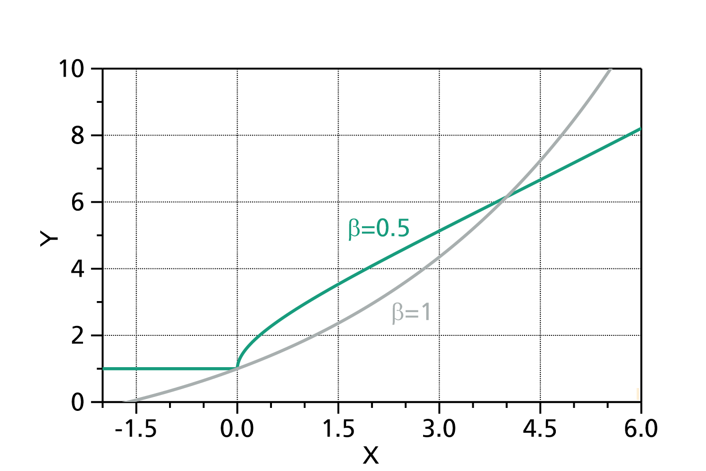
Fig. 1: Stretched exponential growth with ![]() ,
, ![]() ,
, ![]() ,
, ![]() , and
, and ![]() (green) in comparison to a 'normal' exponential growth function with the same parameters (grey). Note that the 'normal' exponential growth has varying function values both for
(green) in comparison to a 'normal' exponential growth function with the same parameters (grey). Note that the 'normal' exponential growth has varying function values both for ![]() and
and ![]() , whereas the stretched exponential growth is constant for
, whereas the stretched exponential growth is constant for ![]() .
.
Two polynomial segments
This function evaluates two polynomial segments that are connected at the point ![]() , according to:
, according to:
in which:
- is the x-coordinate of the point at which the two polynomial segments are joined
- is the y-coordinate of the point at which the two polynomial segments are joined
 are the polynomial coefficients of the left polynomial segment (
 )
)
- ... are the polynomial coefficients of the right polynomial segment (
 )
)
- is the order of the left polynomial segment (
 )
)
- is the order of the right polynomial segment (
 )
)
The polynomial orders ![]() and
and ![]() can be changed by double-clicking on the fit function. The default value is
can be changed by double-clicking on the fit function. The default value is ![]() and
and ![]() , resulting in two straight lines joined at
, resulting in two straight lines joined at ![]() . If some of the terms are not needed, set the corresponding coefficients fixed to zero.
. If some of the terms are not needed, set the corresponding coefficients fixed to zero.
The domain of the function is ![]() .
.
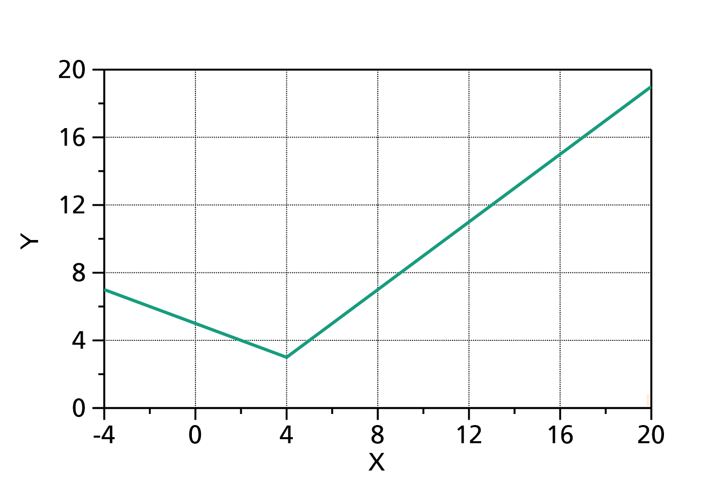
Fig. 1: Two polynomial segments (![]() ,
, ![]() ) with
) with ![]() ,
, ![]() ,
, ![]() and
and ![]() .
.
Conversion of an autocatalytic reaction
This fit function represents the solution of the differential equation for the conversion of an autocatalytic reaction (e.g. epoxy curing), namely:

in which
 is a value in the range [0, 1], e.g. the chemical conversion,
- is the independent variable (for a reaction, represents the time),
 and
and  are a rate parameter,
- and are exponents,
- is the point (time) of the start of the reaction, i.e.
 .
.
Important: In this fit function, the dependent variable
is not the conversion
, but a scaled value of the conversion
, in which
is an additional parameter!
The values of ![]() ,
, ![]() and
and ![]() are assumed to be positive. The value of
are assumed to be positive. The value of ![]() before the start of reaction (
before the start of reaction (![]() ) is assumed to be 0.
) is assumed to be 0.
Since there is no general analytical solution of this differential equation, the solution must be calculated using an ordinary differential equation solver. This could make fits to a large data set somewhat slow.
The domain of the function is ![]() .
.
Tip #1:
To fit conversion data that are in the range [0,1], set the parameter
Tip #2:
To fit conversion data that are in percent, i.e. in a range of [0, 100], set the parameter
Note:
This kinetic equation assumes that the conversion finally reaches 1 (100%). This assumption may be wrong if the glass temperature of the finally cured material exceeds the curing temperature.
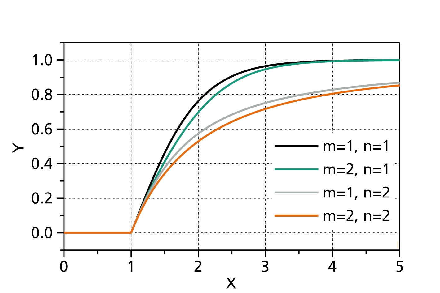
Fig. 1: ConversionAutocatalytic (with ![]() ,
, ![]() ,
, ![]() and
and ![]() =1). The values for
=1). The values for ![]() and
and ![]() are indicated in the legend.
are indicated in the legend.
References:
J. M. Kenny, Determination of Autocatalytic Kinetic Model Parameters Describing Thermoset Cure, Journal of Applied Polymer Science, Vol. 51, 761-764 (1994)
Conversion of a reaction of nth order
This fit function represents the solution of the differential equation of a conversion kinetics of nth order, namely:

in which
- is a value in the range [0, 1], e.g. the chemical conversion,
- is the independent variable (for a kinetics, represents the time),
 is a rate parameter,
- is the order of the kinetic conversion process,
- is the point (time) of the start of the reaction, i.e. .
Important: In this fit function, the dependent variable
The value of ![]() is assumed to be positive.
is assumed to be positive.
The solution for ![]() of the differential equation is:
of the differential equation is:
For ![]() ,
, ![]() is set to 0. Additionally, in order to be consistent among different
is set to 0. Additionally, in order to be consistent among different ![]() ,
, ![]() is set to 1 if
is set to 1 if ![]() and
and ![]() .
.
The domain of the function is ![]() .
.
Tip #1:
To fit conversion data that are in the range [0,1], set the parameter
Tip #2:
To fit conversion data that are in percent, i.e. in a range of [0, 100], set the parameter
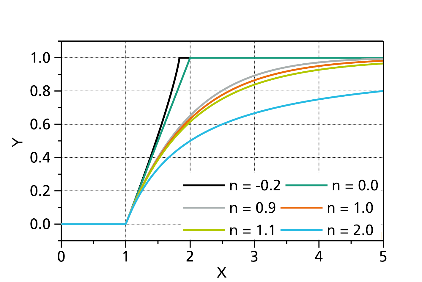
Fig. 1: ConversionNthOrder fit functions (with ![]() ,
, ![]() ,
, ![]() ). The values for
). The values for ![]() are indicated in the legend.
are indicated in the legend.
Kinetics of nth order
This fit function represents the solution of the differential equation for a kinetics of nth order, namely:

in which
- is the dependent variable,
- is the independent variable (for a kinetics, represents the time),
- is a rate parameter,
- is the order of the kinetic process,
- is the value of at .
The values of ![]() and
and ![]() is assumed to be positive.
is assumed to be positive.
The solution of this differential equation is:

The domain of the function is:

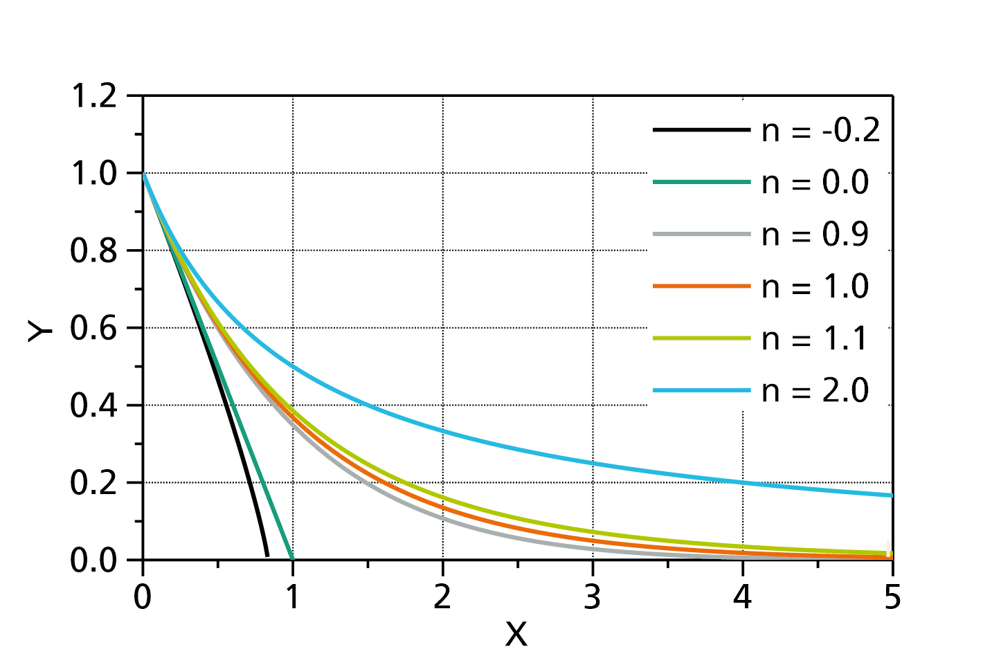
Fig. 1: KineticsNthOrder (with ![]() ,
, ![]() ). The values for
). The values for ![]() are indicated in the legend.
are indicated in the legend.
Rate of conversion of an autocatalytic reaction
This fit function represents the solution of the differential equation for the conversion of an autocatalytic reaction (e.g. epoxy curing), namely:
in which
- is a value in the range [0, 1], e.g. the chemical conversion,
- is the independent variable (for a reaction, represents the time),
- and are a rate parameter,
- and are exponents,
- is the point (time) of the start of the reaction, i.e. .
Important: In this fit function, the dependent variable is not the conversion
, in which
The values of ![]() ,
, ![]() and
and ![]() are assumed to be positive. The value of
are assumed to be positive. The value of ![]() before the start of reaction (
before the start of reaction (![]() ) is assumed to be 0.
) is assumed to be 0.
Since there is no general analytical solution of this differential equation, the solution must be calculated using an ordinary differential equation solver. This could make fits to a large data set somewhat slow.
The domain of the function is ![]() .
.
Note:
This kinetic equation assumes that the conversion finally reaches 1 (100%). This assumption may be wrong if the glass temperature of the finally cured material exceeds the curing temperature.
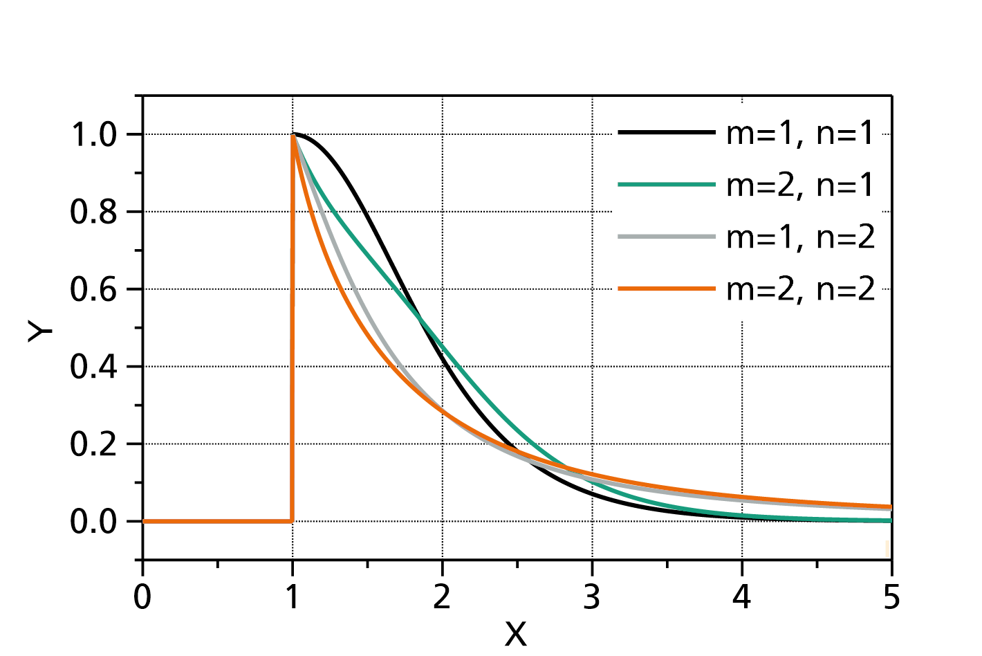
Fig. 1: RateOfConversionAutocatalytic (with ![]() ,
, ![]() ,
, ![]() and
and ![]() =1). The values for
=1). The values for ![]() and
and ![]() are indicated in the legend.
are indicated in the legend.
References:
J. M. Kenny, Determination of Autocatalytic Kinetic Model Parameters Describing Thermoset Cure, Journal of Applied Polymer Science, Vol. 51, 761-764 (1994)
Conversion of a reaction of nth order
This fit function represents the solution of the differential equation of a conversion kinetics of nth order, namely:
in which
- is a value in the range [0, 1], e.g. the chemical conversion,
- is the independent variable (for a kinetics, represents the time),
- is a rate parameter,
- is the order of the kinetic conversion process,
- is the point (time) of the start of the reaction, i.e. .
Important: In this fit function, the dependent variable is not the conversion
The value of ![]() is assumed to be positive.
is assumed to be positive.
The solution for ![]() of the differential equation is:
of the differential equation is:
For ![]() ,
, ![]() is set to 0. Additionally, in order to be consistent among different
is set to 0. Additionally, in order to be consistent among different ![]() ,
, ![]() is set to 1 if
is set to 1 if ![]() and
and ![]() .
.
The domain of the function is ![]() .
.
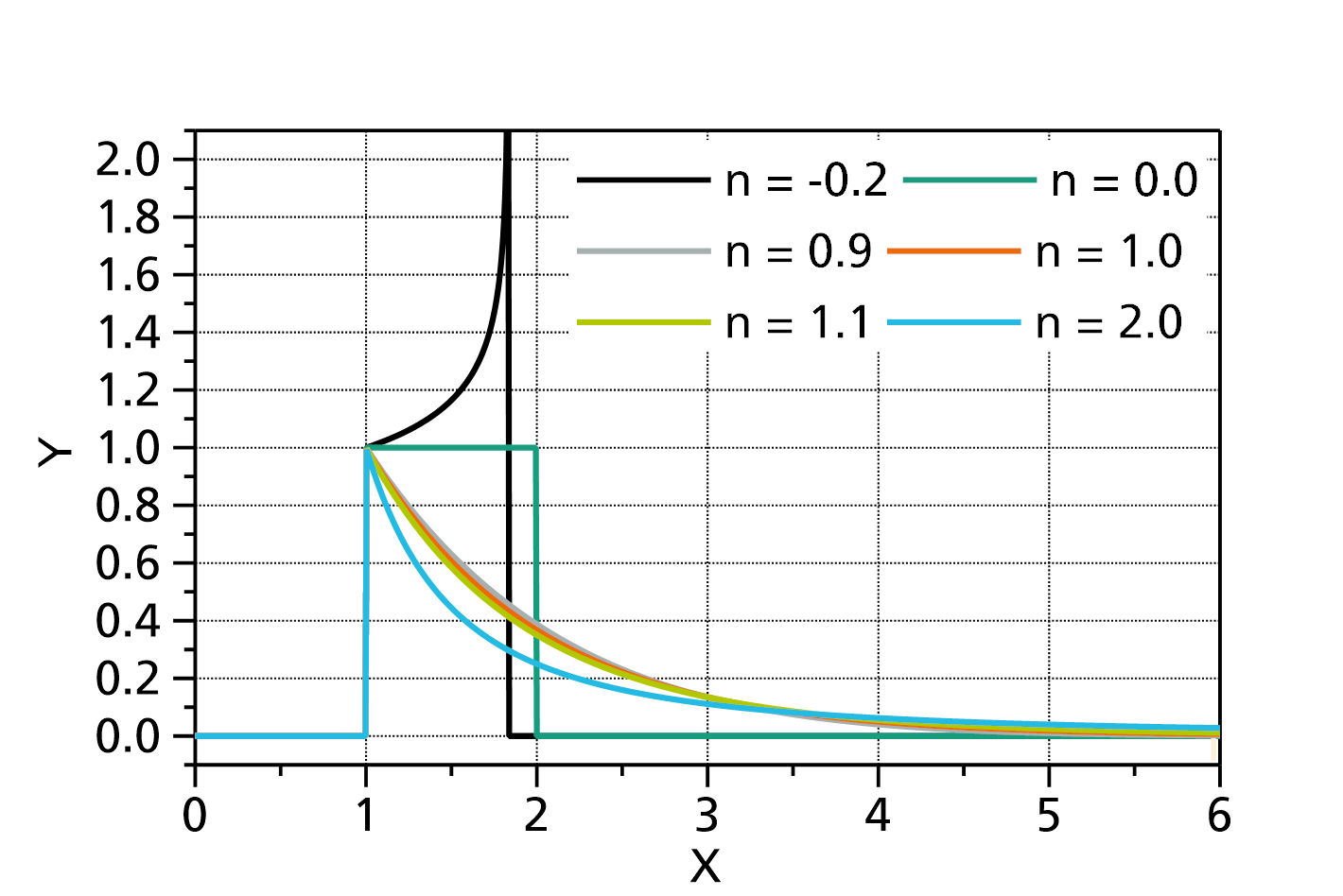
Fig. 1: RateOfConversionNthOrder fit functions (with ![]() ,
, ![]() ,
, ![]() ). The values for
). The values for ![]() are indicated in the legend.
are indicated in the legend.
Arrhenius law (rate)
This Arrhenius law describes the temperature dependence of e.g. reaction rates, typical frequencies, e.g. quantities that increase with increasing temperature.
The function is defined as:
in which ![]() is the reaction rate (dependent variable),
is the reaction rate (dependent variable), ![]() is the absolute (!) temperature (independent variable), and
is the absolute (!) temperature (independent variable), and ![]() is a constant, usually the Boltzmann constant, but it depends on the options you choose for the fit (see below).
is a constant, usually the Boltzmann constant, but it depends on the options you choose for the fit (see below).
The parameters are:
- is the reaction rate in the limit

 is the activation energy.
Please note that for large temperature intervals, the y-value can vary over some orders of magnitude. This will lead to a poor fit, because the data points with small values of the reaction rate then contribute too little to the fit.
In order to get a good fit nevertheless, it is neccessary that you logarithmize your data points before they get fitted, and choose the DecadicLogarithm dependent variable option on this fit.
Options for the independent variable x:
Kelvin: x is
 in Kelvin
AsInverseKelvin: x is

DegreeCelsius: x is in °C
DegreeFahrenheit: x is in °F
Options for the dependent variable y:
Original: the original value of
(the rate)
Inverse: the inverse of the rate, i.e.

Negative: the negative rate

DecadicLogarithm:

NegativeDecadicLogarithm:

NaturalLogarithm:

NegativeNaturalLogarithm:

Option for parameters:
ParameterEnergyRepresentation
Joule:
is in Joule
JoulePerMole:
is in Joule per mole
ElectronVolt:
is in eV (electron volt)
kWh, calorie, calorie per mole and more..
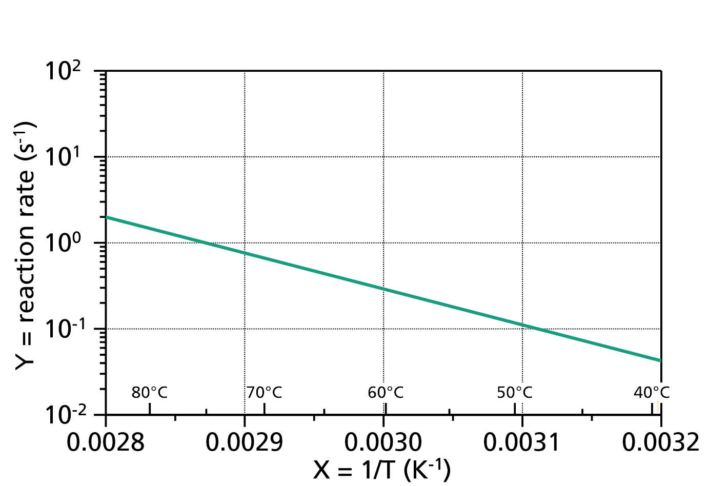
Fig. 1: Typical plot of an Arrhenius diagram (reaction rate by the inverse temperature). Here the parameters are ![]() and
and ![]() kJ/mol. Please note that if you choose the x-axis to be
kJ/mol. Please note that if you choose the x-axis to be ![]() instead of T and the y-axis to be logarithmic, as in this example, the curve becomes a straight line. You can even include the "right" temperatures in °C by adding a second axis at the bottom, with inverse tick spacing and the transformation
instead of T and the y-axis to be logarithmic, as in this example, the curve becomes a straight line. You can even include the "right" temperatures in °C by adding a second axis at the bottom, with inverse tick spacing and the transformation ![]() .
.
Arrhenius law (time)
This Arrhenius law describes the temperature dependence of e.g. relaxation or retardation times, or viscosities, e.g. quantities that decrease with increasing temperature.
The function is defined as:
in which ![]() is the relaxation or retardation time or viscosity (dependent variable),
is the relaxation or retardation time or viscosity (dependent variable), ![]() is the absolute (!) temperature (independent variable), and
is the absolute (!) temperature (independent variable), and ![]() is a constant, usually the Boltzmann constant, but it depends on the options you choose for the fit (see below).
is a constant, usually the Boltzmann constant, but it depends on the options you choose for the fit (see below).
The parameters are:
- is the relaxation or retardation time or viscosity in the limit
- is the activation energy.
Please note that for large temperature intervals, the y-value can vary over some orders of magnitude. This will lead to a poor fit, because the data points with small values of the reaction rate then contribute too little to the fit.
In order to get a good fit nevertheless, it is neccessary that you logarithmize your data points before they get fitted, and choose the DecadicLogarithm dependent variable option on this fit.
Options for the independent variable x:
Kelvin: x is
in Kelvin
AsInverseKelvin: x is
DegreeCelsius: x is in °C
DegreeFahrenheit: x is in °F
Options for the dependent variable y:
Original: the original value of
(the rate)
Inverse: the inverse of the rate, i.e.
Negative: the negative rate
DecadicLogarithm:
NegativeDecadicLogarithm:
NaturalLogarithm:
NegativeNaturalLogarithm:
Option for parameters:
ParameterEnergyRepresentation
Joule:
is in Joule
JoulePerMole:
is in Joule per mole
ElectronVolt:
is in eV (electron volt)
kWh, calorie, calorie per mole and more..
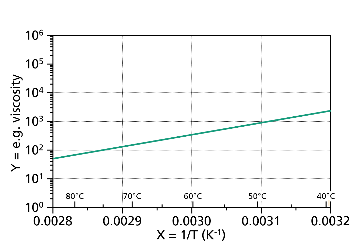
Fig. 1: Typical plot of an Arrhenius diagram (viscosity by the inverse temperature). Here the parameters are ![]() and
and ![]() kJ/mol. Please note that if you choose the x-axis to be
kJ/mol. Please note that if you choose the x-axis to be ![]() instead of T and the y-axis to be logarithmic, as in this example, the curve becomes a straight line. You can even include the "right" temperatures in °C by adding a second axis at the bottom, with inverse tick spacing and the transformation
instead of T and the y-axis to be logarithmic, as in this example, the curve becomes a straight line. You can even include the "right" temperatures in °C by adding a second axis at the bottom, with inverse tick spacing and the transformation ![]() .
.
Vogel-Fulcher law (rate, mobility)
The Vogel-Fulcher law describes the dependence of reaction rates, mobilities, viscosities and relaxation times on the temperature for materials like glasses and polymers for temperatures in the vicinity of the glass transition temperature and in any case above the so-called Vogel temperature ![]() .
.
This variant of the Vogel-Fulcher law is especially suited to describe the temperature dependence of rates, mobilities, diffusion coefficients etc., i.e. quantities which increase with increasing temperatures. in glasses at temperatures above ![]() .
.
The function is defined as:
in which ![]() is the rate, mobility, etc. (dependent variable),
is the rate, mobility, etc. (dependent variable), ![]() is the temperature (independent variable),
is the temperature (independent variable), ![]() is the so-called Vogel temperature, and
is the so-called Vogel temperature, and ![]() is a broadness parameter.
is a broadness parameter.
Note: The function above is designed for reaction rates, mobilities, etc., i.e. for quantities, which increase with increasing temperature. But quantities like viscosity, relaxation times decrease with increasing temperature. To fit those quantities, please use VogelFulcherLaw (Time), or use this function with a negative value for
.
The parameters are:
- is the reaction rate, mobility, ..., etc. in the limit
 is the Vogel-Temperature. The formula is only valid for temperatures
  . At the Vogel temperature, reaction rates, mobilities, etc., converge to zero.
- changes the slope of the curve.
Please note that for large temperature intervals, the function value can vary over many orders of magnitude. This will lead to a poor fit, because the data points with small values then contribute too little to the fit.
In order to get a good fit nevertheless, it is necessary that you logarithmize your data points before they get fitted. In order to do this, choose the DecadicLogarithm or NaturalLogarithm transformation for both the transformation of your data and for the transformation of the fit output ![]() .
.
Options for the independent variable ![]() :
:
Kelvin: Your x-values are absolute temperatures in Kelvin
AsInverseKelvin: your x-values are inverse temperatures
DegreeCelsius: your x-values are given as temperatures in °C
DegreeFahrenheit: your x-values are given as temperatures in °F
Option for parameters:
ParameterEnergyRepresentation
Joule:
is in Joule
JoulePerMole:
is in Joule per mole
ElectronVolt:
is in eV (electron volt)
kWh, calorie, calorie per mole and more..
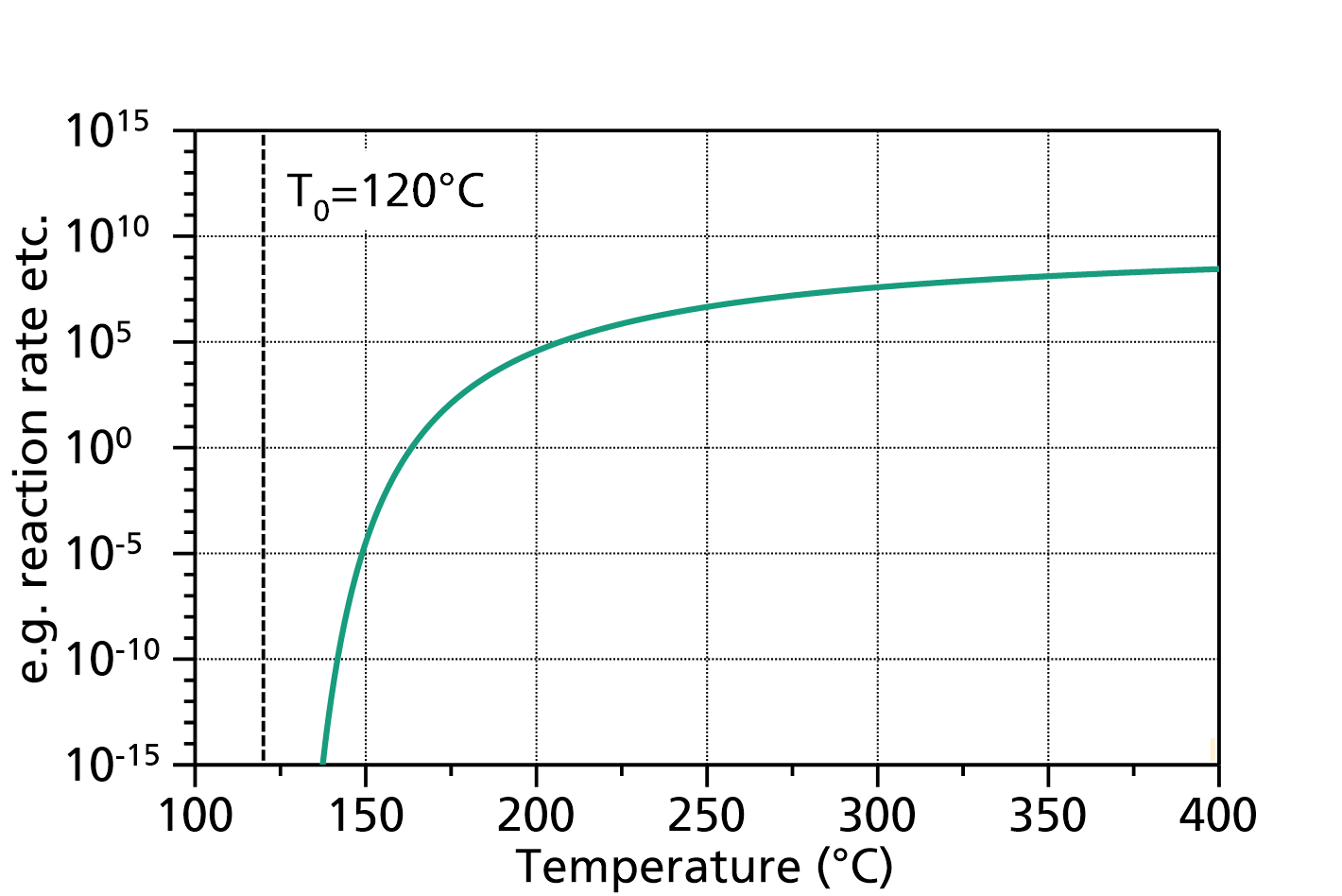
Fig. 1: Vogel-Fulcher law (e.g. reaction rate by temperature). Here the parameters are ![]() ,
, ![]() =120°C and
=120°C and ![]() =1000 K.
=1000 K.
Fig. 2: Vogel-Fulcher law plotted in an Arrhenius diagram (e.g. reaction rate versus inverse temperature). The parameters are ![]() ,
, ![]() =120°C and
=120°C and ![]() =1000 K.
=1000 K.
Vogel-Fulcher law (relaxation times, viscosities)
The Vogel-Fulcher law describes the dependence of reaction rates, mobilities, viscosities and relaxation times on the temperature for materials like glasses and polymers for temperatures in the vicinity of the glass transition temperature and in any case above the so-called Vogel temperature ![]() .
.
This variant of the Vogel-Fulcher law is especially suited to describe the temperature dependence of relaxation times, viscosities, etc., i.e. quantities which decrease with increasing temperatures. in glasses at temperatures above ![]() .
.
The function is defined as:
in which ![]() is the relaxation time, viscosity, etc. (dependent variable),
is the relaxation time, viscosity, etc. (dependent variable), ![]() is the temperature (independent variable),
is the temperature (independent variable), ![]() is the so-called Vogel temperature, and
is the so-called Vogel temperature, and ![]() is a broadness parameter.
is a broadness parameter.
Note: The function above is designed for relaxation times, viscosities, etc, i.e. for quantities, which decrease with increasing temperature. But quantities like reaction rates, mobilities, etc., increase with increasing temperature. To fit those quantities, please use VogelFulcherLawRate, or use this function with a negative value for
The parameters are:
- is the relaxation time, viscosity, ..., etc. in the limit
- is the Vogel-Temperature. The formula is only valid for temperatures . At the Vogel temperature, relaxation times, viscosities, etc., converge to infinity.
- changes the slope of the curve.
Please note that for large temperature intervals, the function value can vary over many orders of magnitude. This will lead to a poor fit, because the data points with small values then contribute too little to the fit.
In order to get a good fit nevertheless, it is necessary that you logarithmize your data points before they get fitted. In order to do this, choose the DecadicLogarithm or NaturalLogarithm transformation for both the transformation of your data and for the transformation of the fit output ![]() .
.
Options for the independent variable ![]() :
:
Kelvin: Your x-values are absolute temperatures in Kelvin
AsInverseKelvin: your x-values are inverse temperatures
DegreeCelsius: your x-values are given as temperatures in °C
DegreeFahrenheit: your x-values are given as temperatures in °F
Option for parameters:
ParameterEnergyRepresentation
Joule:
is in Joule
JoulePerMole:
is in Joule per mole
ElectronVolt:
is in eV (electron volt)
kWh, calorie, calorie per mole and more..
Fig. 1: Vogel-Fulcher law (e.g. relaxation time by temperature). Here the parameters are ![]() ,
, ![]() =120°C and
=120°C and ![]() =1000 K.
=1000 K.
Fig. 2: Vogel-Fulcher law plotted in an Arrhenius diagram (e.g. relaxation time versus inverse temperature). The parameters are ![]() ,
, ![]() =120°C and
=120°C and ![]() =1000 K.
=1000 K.
CauchyAmplitude
This function evaluates a sum of Cauchy (Lorentzian) terms, plus a baseline polynomial with one or multiple terms, according to
in which:
 are the amplitudes (heights) of the Cauchy terms
 are the locations of the Cauchy terms
 are the half widths of half maximum (HWHM) of the Cauchy terms
- are the coefficients of the baseline polynomial of order
- is the number of Cauchy terms ()
- is the order of the baseline polynomial (set to disable the baseline polynomial)
The number of Cauchy terms ![]() and the order of the baseline polynomial
and the order of the baseline polynomial ![]() can be changed by double-clicking on the fit function. The default values are
can be changed by double-clicking on the fit function. The default values are ![]() and
and ![]() .
.
The domain of the function is ![]() .
.
Fig. 1: CauchyAmplitude (![]() ,
, ![]() ) with
) with ![]() ,
, ![]() ,
, ![]() and
and ![]() .
.
References: Cauchy distribution at Wikipedia
GaussAmplitude
This function evaluates a sum of Gaussian terms, plus a baseline polynomial with one or multiple terms, according to
in which:
- are the amplitudes (heights) of the Gaussian terms
- are the locations of the Gaussians
- are the widths of the Gaussians
- are the coefficients of the baseline polynomial of order
- is the number of Gaussian terms ()
- is the order of the baseline polynomial (set to disable the baseline polynomial)
The number of Gaussian terms ![]() and the order of the baseline polynomial
and the order of the baseline polynomial ![]() can be changed by double-clicking on the fit function. The default values are
can be changed by double-clicking on the fit function. The default values are ![]() and
and ![]() .
.
The domain of the function is ![]() .
.

Fig. 1: GaussAmplitude (![]() ,
, ![]() ) with
) with ![]() ,
, ![]() ,
, ![]() and
and ![]() .
.
PearsonIVAmplitude
This function evaluates a sum of PearsonIV terms, plus a baseline polynomial with one or multiple terms, according to
in which:
- are the amplitudes (height of the maxima) of the PearsonIV terms
- are the locations of the PearsonIV terms
- are the widths of the PearsonIV terms
 are the exponents of the PearsonIV terms (
 )
)
 are the skewness parameters of the PearsonIV terms
 are the coefficients of the baseline polynomial of order
- is the number of PearsonIV terms ()
- is the order of the baseline polynomial (set
 to disable the baseline polynomial)
The original PearsonIV function was modified, such as that the location parameters describe the location of the maximal value of the function, and the amplitude parameter is the maximum y-value of the function:
Modified version used in Altaxo:
The number of PearsonIV terms ![]() and the order of the baseline polynomial
and the order of the baseline polynomial ![]() can be changed by double-clicking on the fit function. The default values are
can be changed by double-clicking on the fit function. The default values are ![]() and
and ![]() .
.
The domain of the function is ![]() .
.
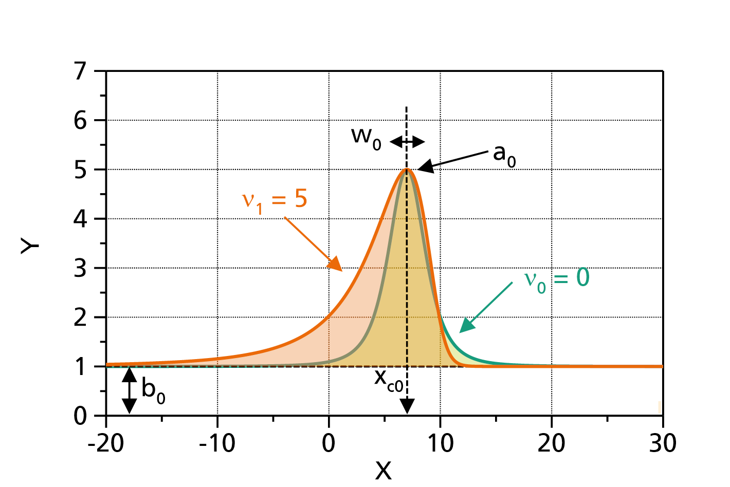
Fig. 1: PearsonIV (![]() ,
, ![]() ) with
) with ![]() ,
, ![]() ,
, ![]() ,
, ![]() ,
, ![]() , and
, and ![]() (green) or
(green) or ![]() (orange), respectively. Note that in the limit
(orange), respectively. Note that in the limit ![]() the PearsonVII function is returned.
the PearsonVII function is returned.
Literature:
[1] Description of the Pearson distribution family in Wikipedia
PearsonIVAmplitude (Parametrization HPW)
This function evaluates a sum of PearsonIV terms, plus a baseline polynomial with one or multiple terms, according to
in which:
- are the amplitudes (height of the maxima) of the PearsonIV terms
- are the locations of the PearsonIV terms
- are the widths of the PearsonIV terms
- are the exponents of the PearsonIV terms ()
- are the skewness parameters of the PearsonIV terms
- are the coefficients of the baseline polynomial of order
- is the number of PearsonIV terms ()
- is the order of the baseline polynomial (set to disable the baselinepolynomial)
The original PearsonIV function was modified, such as that the location parameter ![]() describe the location of the maximal value of the function, the amplitude parameter is the maximum y-value of the function, and the width parameter
describe the location of the maximal value of the function, the amplitude parameter is the maximum y-value of the function, and the width parameter ![]() is the approximate HWHM of the peak:
is the approximate HWHM of the peak:
Modified version used in Altaxo:
The number of PearsonIV terms ![]() and the order of the baseline polynomial
and the order of the baseline polynomial ![]() can be changed by double-clicking on the fit function. The default values are
can be changed by double-clicking on the fit function. The default values are ![]() and
and ![]() .
.
The domain of the function is ![]() .
.
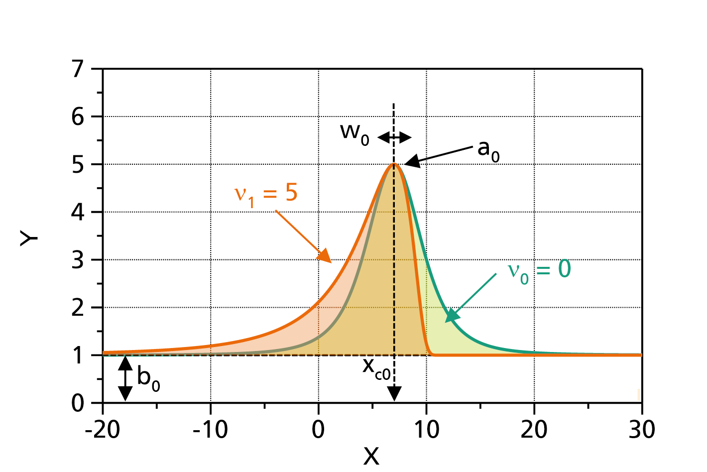
Fig. 1: PearsonIVParametrizationHPW (![]() ,
, ![]() ) with
) with ![]() ,
, ![]() ,
, ![]() ,
, ![]() ,
, ![]() , and
, and ![]() (green) or
(green) or ![]() (orange), respectively. Note that in the limit
(orange), respectively. Note that in the limit ![]() the PearsonVII function (but in another parametrization) is returned.
the PearsonVII function (but in another parametrization) is returned.
Literature:
[1] Description of the Pearson distribution family in Wikipedia
PearsonVIIAmplitude
This function evaluates a sum of PearsonVII terms, plus a baseline polynomial with one or multiple terms, according to
in which:
- are the amplitudes (height of the maxima) of the PearsonVII terms
- are the locations of the PearsonVII terms
- are the widths of the PearsonVII terms
- are the exponents of the PearsonVII terms ()
- are the coefficients of the baseline polynomial of order
- is the number of PearsonVII terms ()
- is the order of the baseline polynomial (set to disable the baseline polynomial)
The PearsonVII function is (see Wikipedia:
The number of PearsonVII terms ![]() and the order of the baseline polynomial
and the order of the baseline polynomial ![]() can be changed by double-clicking on the fit function. The default values are
can be changed by double-clicking on the fit function. The default values are ![]() and
and ![]() .
.
The domain of the function is ![]() .
.
Fig. 1: PearsonVII (![]() ,
, ![]() ) with
) with ![]() ,
, ![]() ,
, ![]() , and
, and ![]() (green) or
(green) or ![]() (orange), respectively. Note that in the limit
(orange), respectively. Note that in the limit ![]() this is the Cauchy function, and in the limit
this is the Cauchy function, and in the limit ![]() a Gaussian.
a Gaussian.
Literature:
[1] Description of the Pearson distribution family in Wikipedia
PseudoVoigt (Amplitude)
This function evaluates a sum of pseudo Voigt terms, plus a baseline polynomial with one or multiple terms, according to
in which:
 are the heights of the pseudo Voigt terms
- are the locations of the pseudo Voigt terms
- are the half-width-half-maximum values (HWHM) of the pseudo Voigt terms
- are the mixing parameters between the Lorentzian part and the Gaussian part
- are the coefficients of the baseline polynomial of order
- is the number of Voigt terms ()
- is the order of the baseline polynomial (set to disable the baseline polynomial)
The pseudo Voigt function is an additive combination of a Gaussian function and a Lorentzian function:
Voigt:
Gauss:
Lorentzian:
The number of pseudo Voigt terms ![]() and the order of the baseline polynomial
and the order of the baseline polynomial ![]() can be changed by double-clicking on the fit function. The default values are
can be changed by double-clicking on the fit function. The default values are ![]() and
and ![]() .
.
The domain of the function is ![]() .
.
Fig. 1: PseudoVoigtAmplitude (![]() ,
, ![]() ) with
) with ![]() ,
, ![]() ,
, ![]() ,
, ![]() , and
, and ![]() (green) or
(green) or ![]() (orange), respectively. Note that in the limit
(orange), respectively. Note that in the limit ![]() the Gauss function is returned, in the limit
the Gauss function is returned, in the limit ![]() the Lorentzian function.
the Lorentzian function.
Shifted Log-Normal (parametrization: NIST)
This function evaluates a sum of shifted log-normal distribution terms, plus a baseline polynomial with one or multiple terms, according to
in which:
is the shifted log-normal function and for which the parametrization is:
- are the heights of the shifted log-normal terms
- are the locations of the maximum of the shifted log-normal terms
- are the full-width-half-maximum values (FWHM) of the shifted log-normal terms
 are skewness parameters of the shifted log-normal terms. The range is
  . For
. For  , the right slope is steeper than the left slope, for
  the left slope is steeper than the right slope. For
  , the shape is Gaussian and therefore symmetric.
- are the coefficients of the baseline polynomial of order
- is the number of shifted log-normal terms ()
- is the order of the baseline polynomial (set to disable the baseline polynomial)
The number of shifted log-normal terms ![]() and the order of the baseline polynomial
and the order of the baseline polynomial ![]() can be changed by double-clicking on the fit function. The default values are
can be changed by double-clicking on the fit function. The default values are ![]() and
and ![]() .
.
For x-values for which the shifted log-normal function is undefined, the y-value of that term is set to zero, so that the resulting domain of the function is ![]() .
.
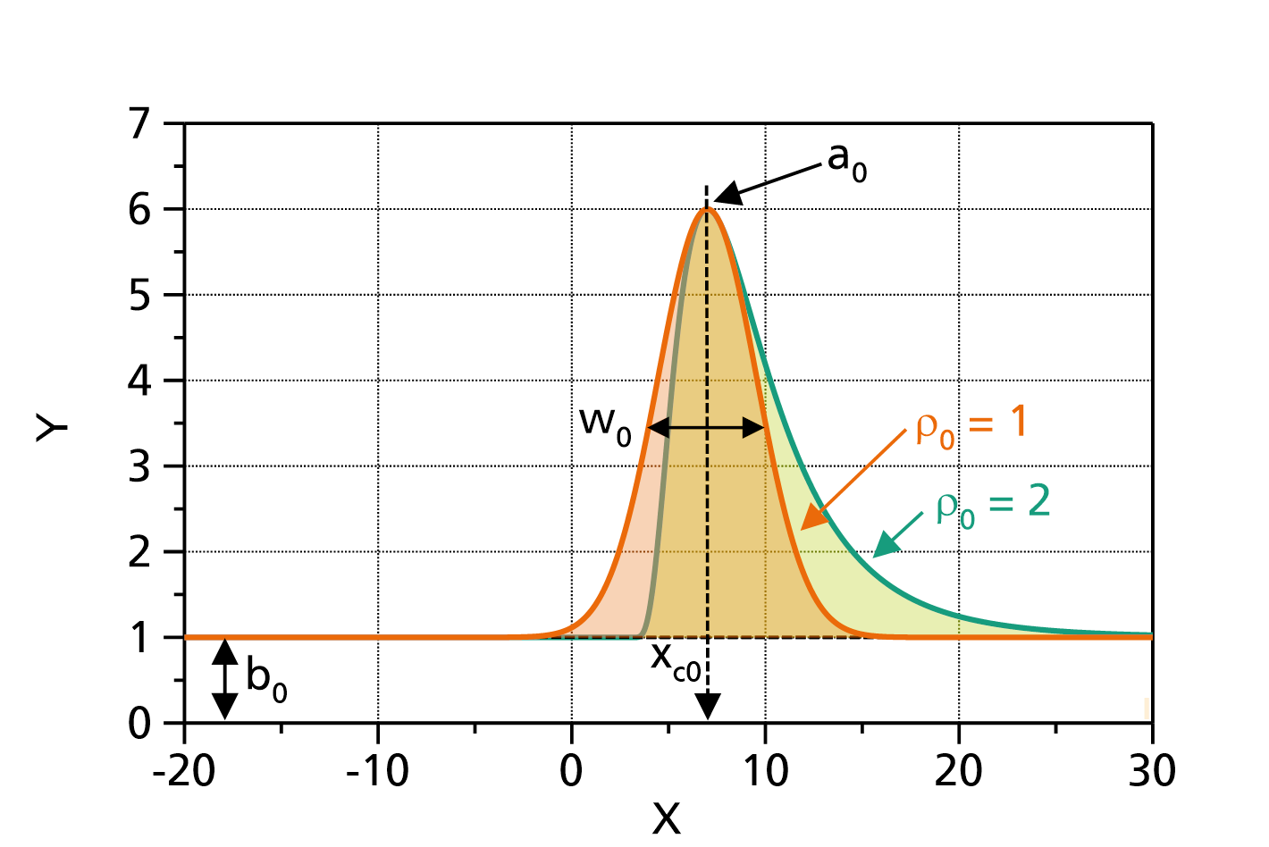
Fig. 1: Shifted log-normal function (![]() ,
, ![]() ) with
) with ![]() ,
, ![]() ,
, ![]() , and
, and ![]() (green) or
(green) or ![]() (orange), respectively. Note that for
(orange), respectively. Note that for ![]() a Gaussian shape is returned.
a Gaussian shape is returned.
Note:
This function is used for instance to describe the intensity in dependence of the Raman shift of the Standard Reference Material 2242a from the National Institute of Standards and Technology NIST. In the formula given in the accompanying document, the number of terms is, and the order of the baseline polynomial is
. The parameter
corresponds to parameter
in the document is the constant background, which is parameter
CauchyArea
This function evaluates a sum of Cauchy (Lorentzian) terms, plus a baseline polynomial with one or multiple terms, according to
in which:
- are the areas under the Cauchy terms
- are the locations of the Cauchy terms
- are the half widths of half maximum (HWHM) of the Cauchy terms
- are the coefficients of the baseline polynomial of order
- is the number of Cauchy terms ()
- is the order of the baseline polynomial (set to disable the baseline polynomial)
The number of Cauchy terms ![]() and the order of the baseline polynomial
and the order of the baseline polynomial ![]() can be changed by double-clicking on the fit function. The default values are
can be changed by double-clicking on the fit function. The default values are ![]() and
and ![]() . In order to get the probability density function of the Cauchy distribution, set
. In order to get the probability density function of the Cauchy distribution, set ![]() ,
, ![]() , and set the parameter
, and set the parameter ![]() fixed to
fixed to ![]() .
.
The domain of the function is ![]() .
.
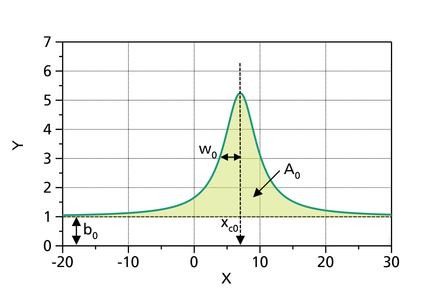
Fig. 1: CauchyArea (![]() ,
, ![]() ) with
) with ![]() ,
, ![]() ,
, ![]() and
and ![]() .
.
References: Cauchy distribution at Wikipedia
GaussArea
This function evaluates a sum of Gaussian terms, plus a baseline polynomial with one or multiple terms, according to
in which:
- are the areas under the Gaussian terms
- are the locations of the Gaussian terms
- are the widths of the Gaussian terms
- are the coefficients of the baseline polynomial of order
- is the number of Gaussian terms ()
- is the order of the baseline polynomial (set to disable the baseline polynomial)
The number of Gaussian terms ![]() and the order of the baseline polynomial
and the order of the baseline polynomial ![]() can be changed by double-clicking on the fit function. The default values are
can be changed by double-clicking on the fit function. The default values are ![]() and
and ![]() .
.
The domain of the function is ![]() .
.
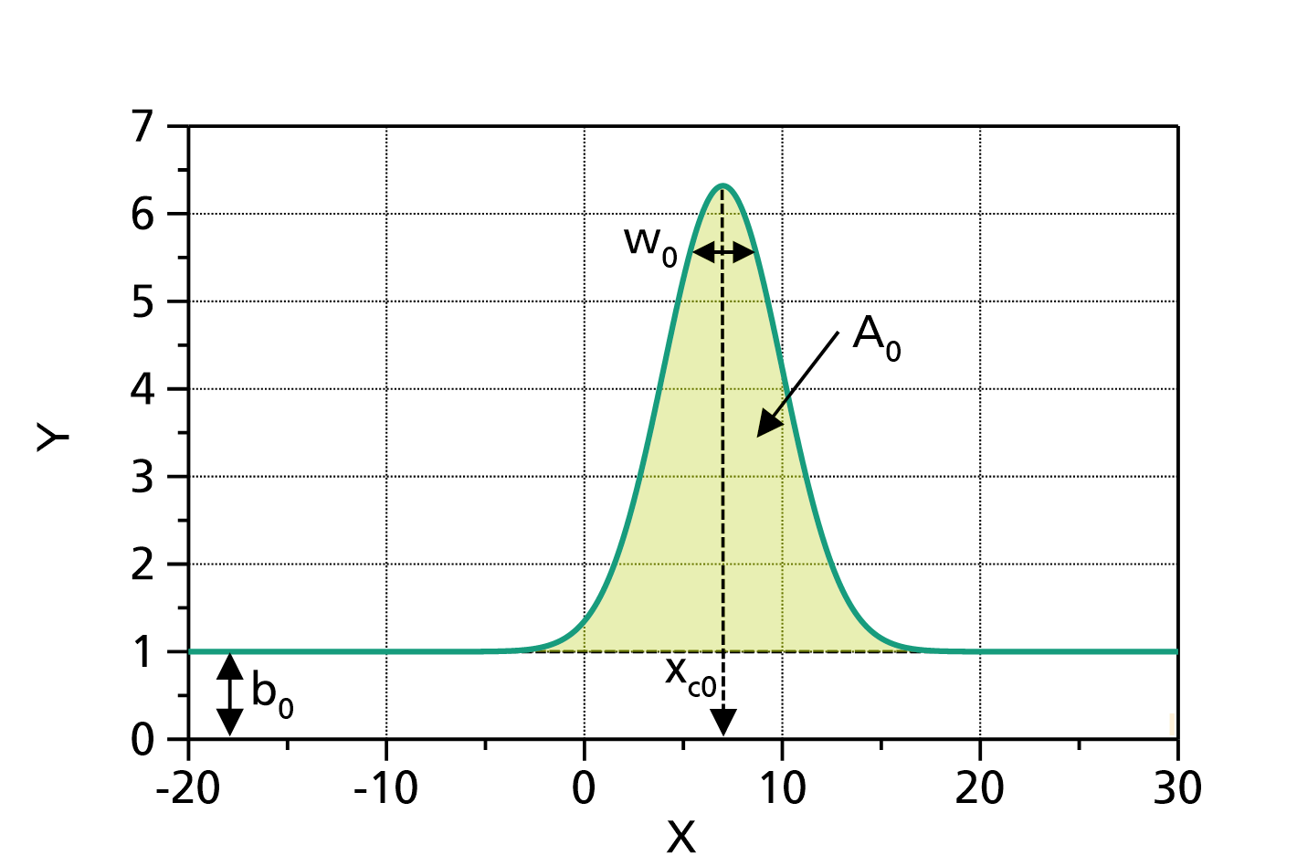
Fig. 1: GaussArea (![]() ,
, ![]() ) with
) with ![]() ,
, ![]() ,
, ![]() and
and ![]() .
.
PearsonIVArea
This function evaluates a sum of PearsonIV terms, plus a baseline polynomial with one or multiple terms, according to
in which:
- are the areas of the PearsonIV terms
- are the location parameters of the PearsonIV terms
- are the widths of the PearsonIV terms
- are the exponents of the PearsonIV terms (
 )
)
- are the skewness parameters of the PearsonIV terms
- are the coefficients of the baseline polynomial of order
- is the number of PearsonIV terms ()
- is the order of the baseline polynomial (set to disable the baseline polynomial)
Please note that the location parameters
are not the location of the maximum function values of the terms! (see figure below)
The PearsonIV function is scaled in a way that its area under the curve is 1:

The location of the maximum function value is at:
The number of PearsonIV terms ![]() and the order of the baseline polynomial
and the order of the baseline polynomial ![]() can be changed by double-clicking on the fit function. The default values are
can be changed by double-clicking on the fit function. The default values are ![]() and
and ![]() .
.
The domain of the function is ![]() .
.
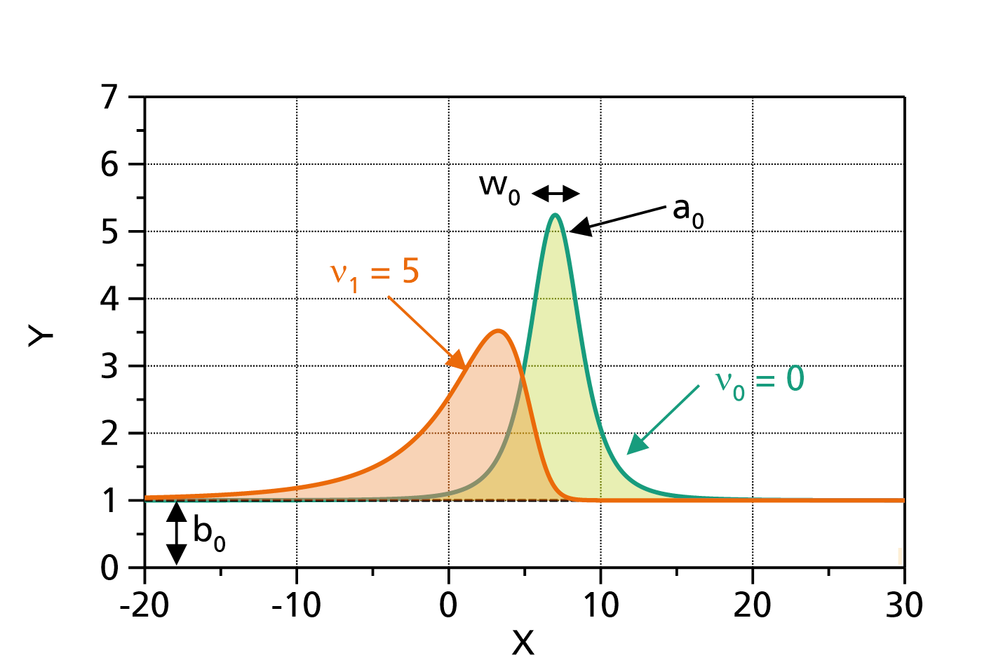
Fig. 1: PearsonIVArea (![]() ,
, ![]() ) with
) with ![]() ,
, ![]() ,
, ![]() ,
, ![]() ,
, ![]() , and
, and ![]() (green) or
(green) or ![]() (orange), respectively. Note that despite the fact that
(orange), respectively. Note that despite the fact that ![]() is equal for both functions, the locations of the maxima are quite different. Only if
is equal for both functions, the locations of the maxima are quite different. Only if ![]() , the location of the maximum function value is
, the location of the maximum function value is ![]() .
.
Literature:
[1] Description of the Pearson distribution family in Wikipedia
VoigtArea
This function evaluates a sum of Voigt terms, plus a baseline polynomial with one or multiple terms, according to
in which:
- are the areas under the Voigt terms
- are the locations of the Voigt terms
- are the widths of the Gaussian part of the Voigt terms
 are the parameters of the Lorentzian part of the Voigt terms
- are the coefficients of the baseline polynomial of order
- is the number of Voigt terms ()
- is the order of the baseline polynomial (set to disable the baseline polynomial)
The Voigt function is a convolution of a Gaussian function and a Lorentzian function:
Voigt:
Gauss:
Lorentzian:
The number of Voigt terms ![]() and the order of the baseline polynomial
and the order of the baseline polynomial ![]() can be changed by double-clicking on the fit function. The default values are
can be changed by double-clicking on the fit function. The default values are ![]() and
and ![]() .
.
The domain of the function is ![]() .
.
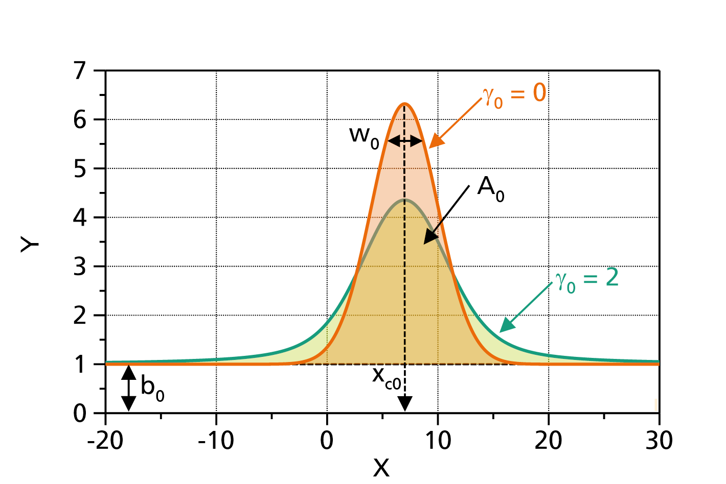
Fig. 1: VoigtArea (![]() ,
, ![]() ) with
) with ![]() ,
, ![]() ,
, ![]() ,
, ![]() , and
, and ![]() (green) or
(green) or ![]() (orange), respectively. Note that in the limit
(orange), respectively. Note that in the limit ![]() the Gauss function is returned.
the Gauss function is returned.
VoigtArea (Parametrization Nu)
This function evaluates a sum of Voigt terms, plus a baseline polynomial with one or multiple terms, according to
in which:
- are the areas under the Voigt terms
- are the locations of the Voigt terms
- are the approximate half-width-half-maximum (HWHM) values of the peaks
- are the mixing parameters (range: 0..1) that determine the Lorentzian'ness or Gauss'ness of the terms
- are the coefficients of the background polynomial of order
- is the number of Voigt terms ()
- is the order of the baseline polynomial (set to disable the baseline polynomial)
The original definition of the Voigt function is a convolution of a Gaussian function and a Lorentzian function:
Voigt:
Gauss:
Lorentzian:
Here, another parametrization with the two parameters ![]() and
and ![]() is used. The new parameters are related to the original parameters
is used. The new parameters are related to the original parameters ![]() by:
by:
Parameter ![]() is the approximate HWHM of the peak, and parameter
is the approximate HWHM of the peak, and parameter ![]() (
(![]() ) determines the ratio between
) determines the ratio between ![]() and
and ![]() , i.e. whether the peak is more Lorentzian like (
, i.e. whether the peak is more Lorentzian like (![]() ) or more Gauss like (
) or more Gauss like (![]() ).
This parametrization is preferred over the original Voigt function if fitting with parameter constraints is performed.
).
This parametrization is preferred over the original Voigt function if fitting with parameter constraints is performed.
The number of Voigt terms ![]() and the order of the baseline polynomial
and the order of the baseline polynomial ![]() can be changed by double-clicking on the fit function. The default values are
can be changed by double-clicking on the fit function. The default values are ![]() and
and ![]() .
.
The domain of the function is ![]() .
.
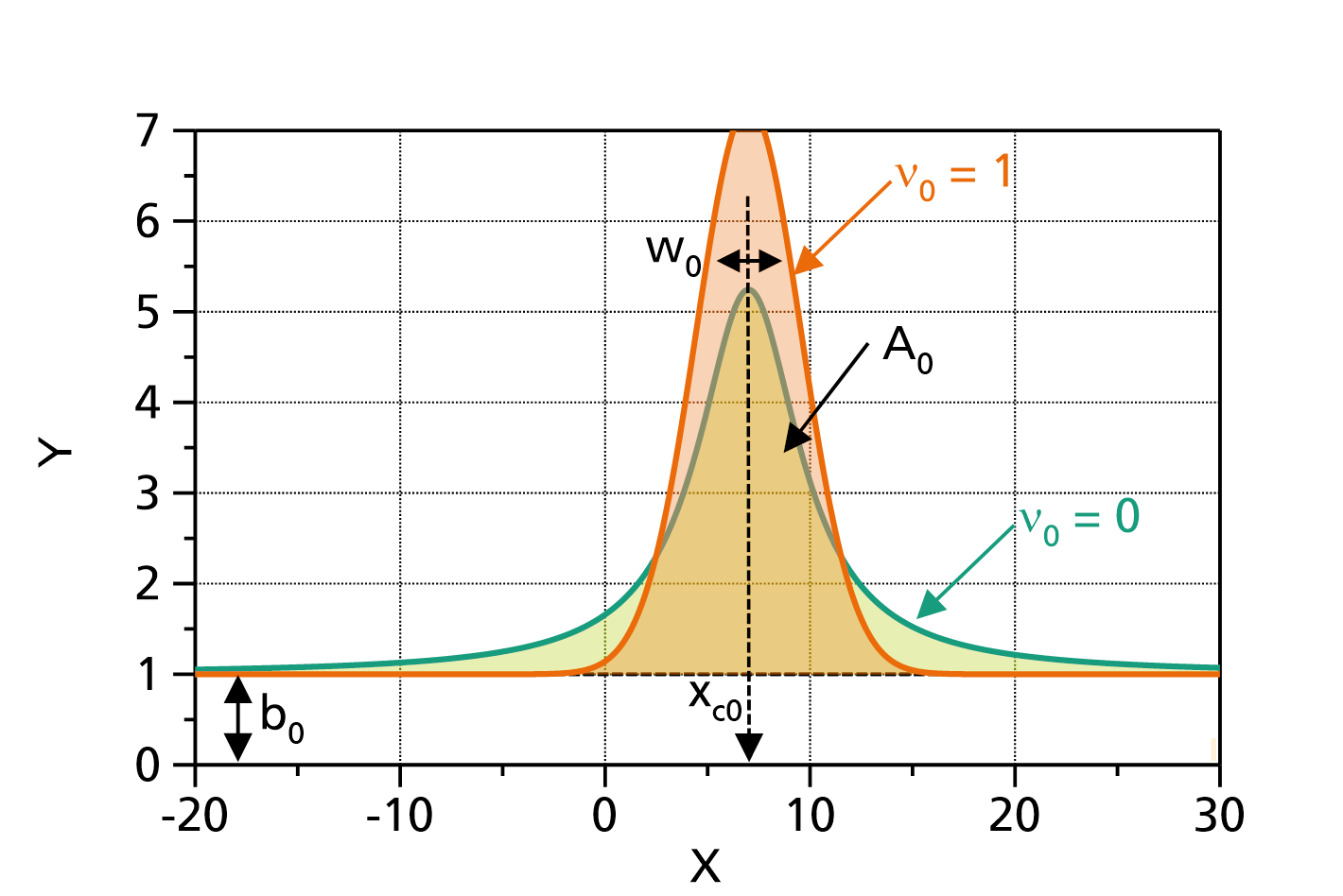
Fig. 1: VoigtAreaParametrizationNu (![]() ,
, ![]() ) with
) with ![]() ,
, ![]() ,
, ![]() ,
, ![]() , and
, and ![]() (green) or
(green) or ![]() (orange), respectively. Note that in the limit
(orange), respectively. Note that in the limit ![]() the peak is a Lorentzian, in the limit of
the peak is a Lorentzian, in the limit of ![]() the peak is a Gaussian.
the peak is a Gaussian.
Modulus relaxation fit functions
Havriliak-Negami modulus relaxation (circular frequency)
This function models the complex dynamic modulus in dependence on the frequency as:
or with a generalized flow term (both equations are equivalent if ![]() ) :
) :
with the frequency ![]() being the independent variable, and
being the independent variable, and ![]() and
and ![]() being the dependent variables, namely the real and imaginary part of the complex dynamic modulus
being the dependent variables, namely the real and imaginary part of the complex dynamic modulus ![]() .
.
The parameters are:
- : low frequency modulus limit
 : high frequency modulus limit
- : relaxation time
 ,
,  : shape exponents (usually
  and
and  )
)
- : generalized flow term, for instance fluidity (inverse viscosity), conductivity etc.
Note:
Since in most cases

Fig. 1: Havriliak-Negami (with ![]() ,
, ![]() ,
, ![]() and
and ![]() ). The values for
). The values for ![]() and
and ![]() are indicated in the legend.
are indicated in the legend.
Fig. 2: Comparison of Havriliak-Negami (with ![]() ,
, ![]() ,
, ![]() ,
, ![]() and
and ![]() ) without and with flow term. The values for
) without and with flow term. The values for ![]() are indicated in the legend.
are indicated in the legend.
References:
Havriliak, S., Negami, S., "A complex plane representation of dielectric and mechanical relaxation processes in some polymers", Polymer 8: 161–210, doi:10.1016/0032-3861(67)90021-3
Havriliak-Negami modulus relaxation (circular frequency)
This function models the complex dynamic modulus in dependence on the circular frequency as:
or with a generalized flow term (both equations are equivalent if ![]() ) :
) :
with the circular frequency ![]() being the independent variable, and
being the independent variable, and ![]() and
and ![]() being the dependent variables, namely the real and imaginary part of the complex dynamic modulus
being the dependent variables, namely the real and imaginary part of the complex dynamic modulus ![]() .
.
The parameters are:
- : low frequency modulus limit
- : high frequency modulus limit
- : relaxation time
- , : shape exponents (usually and )
- : generalized flow term, for instance fluidity (inverse viscosity), conductivity etc.
Note:
Since in most cases

Fig. 1: Havriliak-Negami (with ![]() ,
, ![]() ,
, ![]() and
and ![]() ). The values for
). The values for ![]() and
and ![]() are indicated in the legend.
are indicated in the legend.
Fig. 2: Comparison of Havriliak-Negami (with ![]() ,
, ![]() ,
, ![]() ,
, ![]() and
and ![]() ) without and with flow term. The values for
) without and with flow term. The values for ![]() are indicated in the legend.
are indicated in the legend.
References:
Havriliak, S., Negami, S., "A complex plane representation of dielectric and mechanical relaxation processes in some polymers", Polymer 8: 161–210, doi:10.1016/0032-3861(67)90021-3
Kohlrausch modulus relaxation (frequency)
This function models the complex dynamic modulus in dependence on the frequency as:

or with a generalized flow term (both equations are equivalent if ![]() ) :
) :

based on the Fourier transform of the derivative of the time-domain Kohlrausch function ![]() .
.
The quantities are described below. It is a special case of the underlying base function with the options UseFrequencyInsteadOfOmega=true, UseFlowTerm=true, InvertViscosity=false and LogarithmizeResult=false. These options can be changed by double-clicking on the fit function.
The underlying base function models the generalized complex dynamic modulus in dependence on the circular frequency ![]() with one relaxation term and a flow term as:
with one relaxation term and a flow term as:

based on the Fourier transformation of the time derivative of the Kohlrausch function ![]() , with the circular frequency
, with the circular frequency ![]() being the independent variable (or, depending on an option, the frequency
being the independent variable (or, depending on an option, the frequency ![]() ,
, ![]() ), and
), and ![]() and
and ![]() being the dependent variables, namely the real and negative imaginary part of the complex dynamic modulus
being the dependent variables, namely the real and negative imaginary part of the complex dynamic modulus ![]() .
.
Typical use cases are fits to the complex to the complex mechanical modulus ![]() (e.g. shear modulus
(e.g. shear modulus ![]() or Young's modulus
or Young's modulus ![]() )
)
The parameters are:
- : low frequency modulus limit
- : high frequency modulus limit
- : relaxation time
 : shape exponent (usually )
- : fluidity (inverse viscosity)
 : viscosity
The available options are:
UseFrequencyInsteadOfOmega:
If true, the frequency is used as the independent variable, thus
  in the formula above is replaced by
  .
.
If false, the circular frequency () is used as the independent variable.
UseFlowTerm:
If true, the flow term in above formula is used.
If false, the flow term is not used, and the parameter corresponding with the flow term will not show in the fit.InvertViscosity:
If true, the parameter in the flow term is an inverted viscosity (i.e. fluidity). Thus the flow term generally is .
.
If false, the parameter in the flow term is a viscosity, and the flow term generally is .
.
LogarithmizeResult:
If true, the resulting values of and
and  are logarithmized (decadic logarithm).
If false, the original values are used.
Note:
Since in most cases
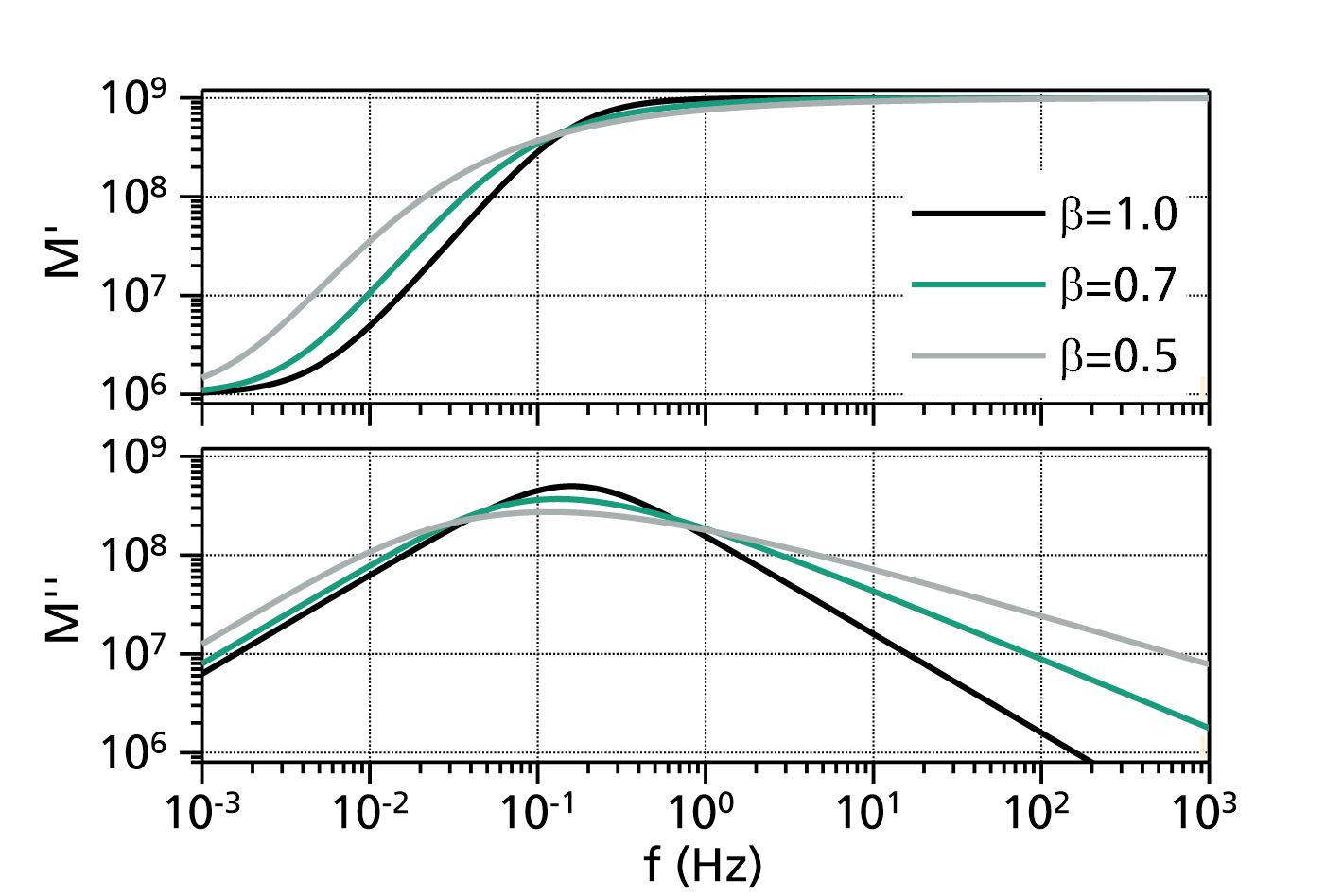
Fig. 1: Kohlrausch fit functions (with ![]() ,
, ![]() ,
, ![]() and
and ![]() ). The values for
). The values for ![]() are indicated in the legend.
are indicated in the legend.
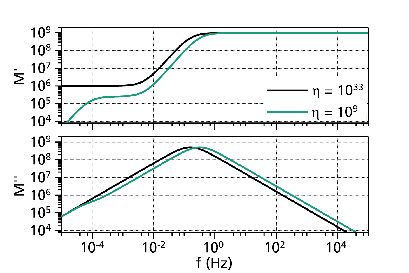
Fig. 2: Comparison of Kohlrausch fit functions (with ![]() ,
, ![]() ,
, ![]() and
and ![]() ) without and with flow term. The values for
) without and with flow term. The values for ![]() are indicated in the legend.
are indicated in the legend.
References:
Kohlrausch, R., "Theorie des elektrischen Rückstandes in der Leidner Flasche", Annalen der Physik und Chemie. 91 (1) (1854): 56–82, 179–213, doi:10.1002/andp.18541670103
Williams, G., Watts, D. C., "Non-Symmetrical Dielectric Relaxation Behavior Arising from a Simple Empirical Decay Function", Transactions of the Faraday Society 66 (1970) 80–85. doi:10.1039/tf9706600080
Kohlrausch modulus relaxation (circular frequency)
This function models the complex dynamic modulus in dependence on the circular frequency as:

or with a generalized flow term (both equations are equivalent if ![]() ) :
) :

based on the Fourier transform of the derivative of the time-domain Kohlrausch function ![]() .
.
The quantities are described below. It is a special case of the underlying base function with the options UseFrequencyInsteadOfOmega=false, UseFlowTerm=true, InvertViscosity=false and LogarithmizeResult=false. These options can be changed by double-clicking on the fit function.
The underlying base function models the generalized complex dynamic modulus in dependence on the circular frequency ![]() with one relaxation term and a flow term as:
with one relaxation term and a flow term as:
based on the Fourier transformation of the time derivative of the Kohlrausch function ![]() , with the circular frequency
, with the circular frequency ![]() being the independent variable (or, depending on an option, the frequency
being the independent variable (or, depending on an option, the frequency ![]() ,
, ![]() ), and
), and ![]() and
and ![]() being the dependent variables, namely the real and negative imaginary part of the complex dynamic modulus
being the dependent variables, namely the real and negative imaginary part of the complex dynamic modulus ![]() .
.
Typical use cases are fits to the complex to the complex mechanical modulus ![]() (e.g. shear modulus
(e.g. shear modulus ![]() or Young's modulus
or Young's modulus ![]() )
)
The parameters are:
- : low frequency modulus limit
- : high frequency modulus limit
- : relaxation time
- : shape exponent (usually )
- : fluidity (inverse viscosity)
- : viscosity
The available options are:
UseFrequencyInsteadOfOmega:
If true, the frequency is used as the independent variable, thus in the formula above is replaced by .
If false, the circular frequency () is used as the independent variable.
UseFlowTerm:
If true, the flow term in above formula is used.
If false, the flow term is not used, and the parameter corresponding with the flow term will not show in the fit.InvertViscosity:
If true, the parameter in the flow term is an inverted viscosity (i.e. fluidity). Thus the flow term generally is.
If false, the parameter in the flow term is a viscosity, and the flow term generally is.
LogarithmizeResult:
If true, the resulting values of and are logarithmized (decadic logarithm).
If false, the original values are used.
Note:
Since in most cases
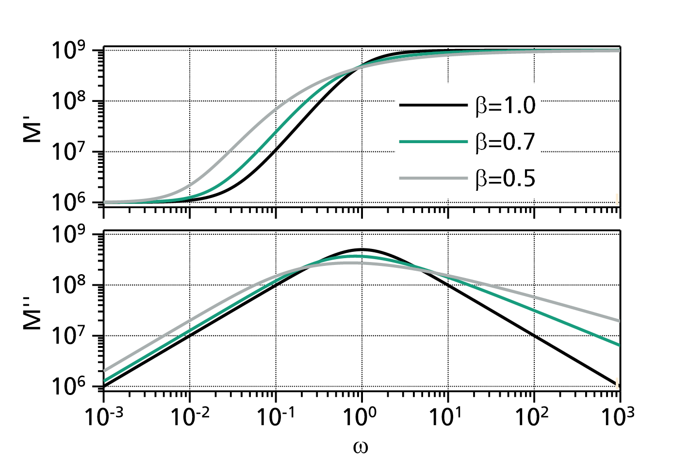
Fig. 1: Kohlrausch fit functions (with ![]() ,
, ![]() ,
, ![]() and
and ![]() ). The values for
). The values for ![]() are indicated in the legend.
are indicated in the legend.
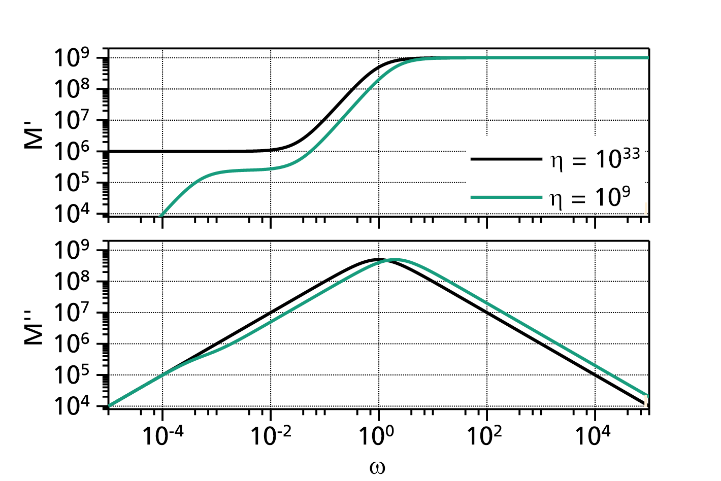
Fig. 2: Comparison of Kohlrausch fit functions (with ![]() ,
, ![]() ,
, ![]() and
and ![]() ) without and with flow term. The values for
) without and with flow term. The values for ![]() are indicated in the legend.
are indicated in the legend.
References:
Kohlrausch, R., "Theorie des elektrischen Rückstandes in der Leidner Flasche", Annalen der Physik und Chemie. 91 (1) (1854): 56–82, 179–213, doi:10.1002/andp.18541670103
Williams, G., Watts, D. C., "Non-Symmetrical Dielectric Relaxation Behavior Arising from a Simple Empirical Decay Function", Transactions of the Faraday Society 66 (1970) 80–85. doi:10.1039/tf9706600080
Havriliak-Negami modulus relaxation (frequency)
This function models the complex dynamic modulus in dependence on the frequency as:
or with a generalized flow term (both equations are equivalent if ![]() ) :
) :
with the frequency ![]() being the independent variable, and
being the independent variable, and ![]() and
and ![]() being the dependent variables, namely the decadic logarithm of the real and imaginary part of the complex dynamic modulus
being the dependent variables, namely the decadic logarithm of the real and imaginary part of the complex dynamic modulus ![]() .
.
The parameters are:
- : low frequency modulus limit
- : high frequency modulus limit
- : relaxation time
- , : shape exponents (usually and )
- : generalized flow term, for instance fluidity (inverse viscosity), conductivity etc.
Note:
If your data are not logarithmized already, please use a DecadicLogarithmTransformation for your data.
Fig. 1: Havriliak-Negami (with ![]() ,
, ![]() ,
, ![]() and
and ![]() ). The values for
). The values for ![]() and
and ![]() are indicated in the legend.
are indicated in the legend.
Fig. 2: Comparison of Havriliak-Negami (with ![]() ,
, ![]() ,
, ![]() ,
, ![]() and
and ![]() ) without and with flow term. The values for
) without and with flow term. The values for ![]() are indicated in the legend.
are indicated in the legend.
References:
Havriliak, S., Negami, S., "A complex plane representation of dielectric and mechanical relaxation processes in some polymers", Polymer 8: 161–210, doi:10.1016/0032-3861(67)90021-3
Havriliak-Negami modulus relaxation (circular frequency)
This function models the complex dynamic modulus in dependence on the circular frequency as:
or with a generalized flow term (both equations are equivalent if ![]() ) :
) :
with the circular frequency ![]() being the independent variable, and
being the independent variable, and ![]() and
and ![]() being the dependent variables, namely the decadic logarithm of the real and imaginary part of the complex dynamic modulus
being the dependent variables, namely the decadic logarithm of the real and imaginary part of the complex dynamic modulus ![]() .
.
The parameters are:
- : low frequency modulus limit
- : high frequency modulus limit
- : relaxation time
- , : shape exponents (usually and )
- : generalized flow term, for instance fluidity (inverse viscosity), conductivity etc.
Note:
If your data are not logarithmized already, please use a DecadicLogarithmTransformation for your data.

Fig. 1: Havriliak-Negami (with ![]() ,
, ![]() ,
, ![]() and
and ![]() ). The values for
). The values for ![]() and
and ![]() are indicated in the legend.
are indicated in the legend.
Fig. 2: Comparison of Havriliak-Negami (with ![]() ,
, ![]() ,
, ![]() ,
, ![]() and
and ![]() ) without and with flow term. The values for
) without and with flow term. The values for ![]() are indicated in the legend.
are indicated in the legend.
References:
Havriliak, S., Negami, S., "A complex plane representation of dielectric and mechanical relaxation processes in some polymers", Polymer 8: 161–210, doi:10.1016/0032-3861(67)90021-3
Kohlrausch modulus relaxation (frequency)
This function models the complex dynamic modulus in dependence on the frequency as:
or with a generalized flow term (both equations are equivalent if ![]() ) :
) :
based on the Fourier transform of the derivative of the time-domain Kohlrausch function ![]() .
.
Here, the values of the real and imaginary part of the calculated modulus are logarithmized for the output:
Should your data are not logarithmized, use a DecadicLogarithmTransformation to logarithmize them, too.
The quantities are described below. It is a special case of the underlying base function with the options UseFrequencyInsteadOfOmega=true, UseFlowTerm=true, InvertViscosity=false and LogarithmizeResult=false. These options can be changed by double-clicking on the fit function.
The underlying base function models the generalized complex dynamic modulus in dependence on the circular frequency ![]() with one relaxation term and a flow term as:
with one relaxation term and a flow term as:
based on the Fourier transformation of the time derivative of the Kohlrausch function ![]() , with the circular frequency
, with the circular frequency ![]() being the independent variable (or, depending on an option, the frequency
being the independent variable (or, depending on an option, the frequency ![]() ,
, ![]() ), and
), and ![]() and
and ![]() being the dependent variables, namely the real and negative imaginary part of the complex dynamic modulus
being the dependent variables, namely the real and negative imaginary part of the complex dynamic modulus ![]() .
.
Typical use cases are fits to the complex to the complex mechanical modulus ![]() (e.g. shear modulus
(e.g. shear modulus ![]() or Young's modulus
or Young's modulus ![]() )
)
The parameters are:
- : low frequency modulus limit
- : high frequency modulus limit
- : relaxation time
- : shape exponent (usually )
- : fluidity (inverse viscosity)
- : viscosity
The available options are:
UseFrequencyInsteadOfOmega:
If true, the frequency is used as the independent variable, thus in the formula above is replaced by .
If false, the circular frequency () is used as the independent variable.
UseFlowTerm:
If true, the flow term in above formula is used.
If false, the flow term is not used, and the parameter corresponding with the flow term will not show in the fit.InvertViscosity:
If true, the parameter in the flow term is an inverted viscosity (i.e. fluidity). Thus the flow term generally is.
If false, the parameter in the flow term is a viscosity, and the flow term generally is.
LogarithmizeResult:
If true, the resulting values of and are logarithmized (decadic logarithm).
If false, the original values are used.
Note:
Since in most cases
Fig. 1: Kohlrausch fit functions (with ![]() ,
, ![]() ,
, ![]() and
and ![]() ). The values for
). The values for ![]() are indicated in the legend.
are indicated in the legend.
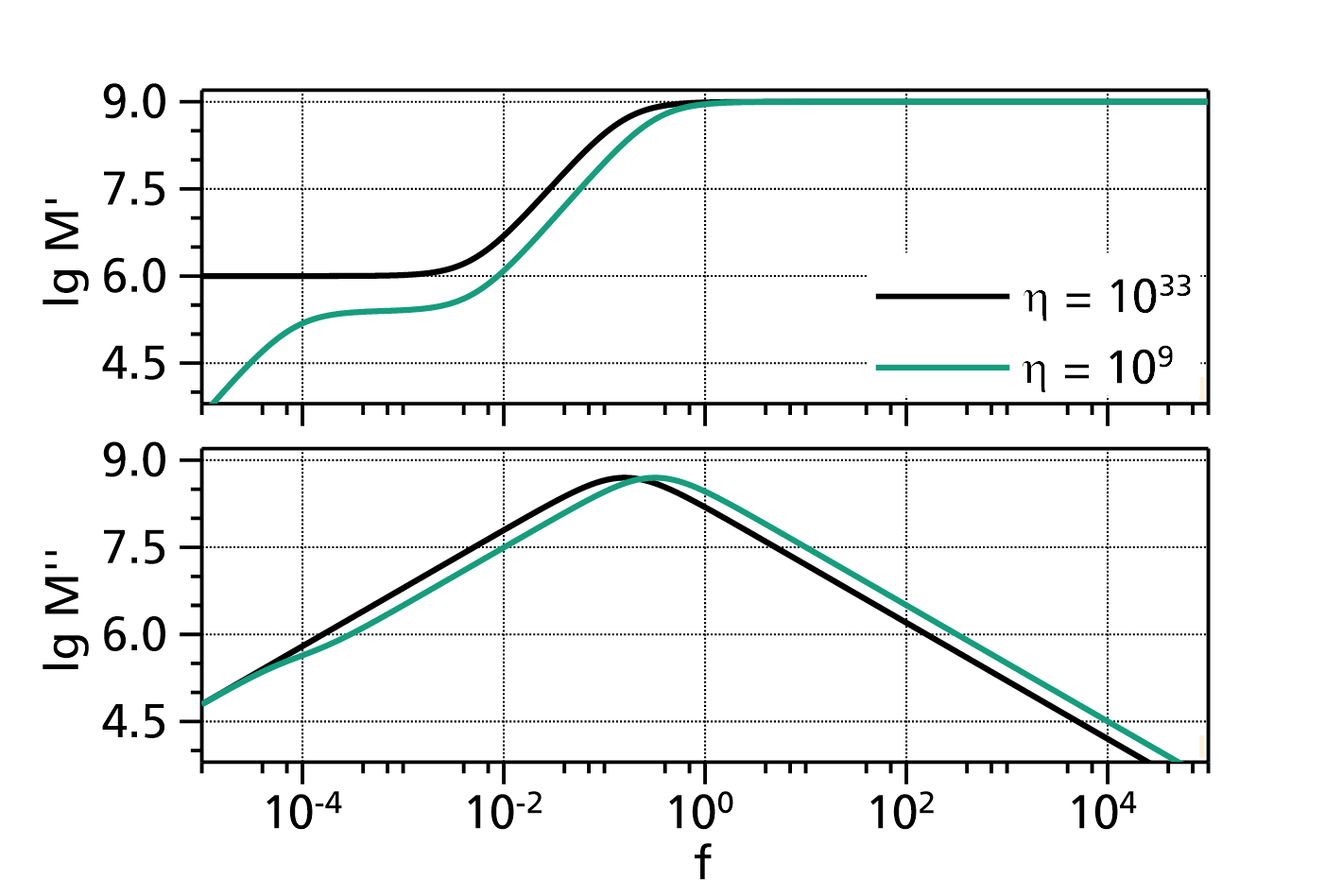
Fig. 2: Comparison of Kohlrausch fit functions (with ![]() ,
, ![]() ,
, ![]() and
and ![]() ) without and with flow term. The values for
) without and with flow term. The values for ![]() are indicated in the legend.
are indicated in the legend.
References:
Kohlrausch, R., "Theorie des elektrischen Rückstandes in der Leidner Flasche", Annalen der Physik und Chemie. 91 (1) (1854): 56–82, 179–213, doi:10.1002/andp.18541670103
Williams, G., Watts, D. C., "Non-Symmetrical Dielectric Relaxation Behavior Arising from a Simple Empirical Decay Function", Transactions of the Faraday Society 66 (1970) 80–85. doi:10.1039/tf9706600080
Kohlrausch modulus relaxation (circular frequency)
This function models the complex dynamic modulus in dependence on the circular frequency as:
or with a generalized flow term (both equations are equivalent if ![]() ) :
) :
based on the Fourier transform of the derivative of the time-domain Kohlrausch function ![]() .
.
Here, the values of the real and imaginary part of the calculated modulus are logarithmized for the output:
Should your data are not logarithmized, use a DecadicLogarithmTransformation to logarithmize them, too.
The quantities are described below. It is a special case of the underlying base function with the options UseFrequencyInsteadOfOmega=false, UseFlowTerm=true, InvertViscosity=false and LogarithmizeResult=false. These options can be changed by double-clicking on the fit function.
The underlying base function models the generalized complex dynamic modulus in dependence on the circular frequency ![]() with one relaxation term and a flow term as:
with one relaxation term and a flow term as:
based on the Fourier transformation of the time derivative of the Kohlrausch function ![]() , with the circular frequency
, with the circular frequency ![]() being the independent variable (or, depending on an option, the frequency
being the independent variable (or, depending on an option, the frequency ![]() ,
, ![]() ), and
), and ![]() and
and ![]() being the dependent variables, namely the real and negative imaginary part of the complex dynamic modulus
being the dependent variables, namely the real and negative imaginary part of the complex dynamic modulus ![]() .
.
Typical use cases are fits to the complex to the complex mechanical modulus ![]() (e.g. shear modulus
(e.g. shear modulus ![]() or Young's modulus
or Young's modulus ![]() )
)
The parameters are:
- : low frequency modulus limit
- : high frequency modulus limit
- : relaxation time
- : shape exponent (usually )
- : fluidity (inverse viscosity)
- : viscosity
The available options are:
UseFrequencyInsteadOfOmega:
If true, the frequency is used as the independent variable, thus in the formula above is replaced by .
If false, the circular frequency () is used as the independent variable.
UseFlowTerm:
If true, the flow term in above formula is used.
If false, the flow term is not used, and the parameter corresponding with the flow term will not show in the fit.InvertViscosity:
If true, the parameter in the flow term is an inverted viscosity (i.e. fluidity). Thus the flow term generally is.
If false, the parameter in the flow term is a viscosity, and the flow term generally is.
LogarithmizeResult:
If true, the resulting values of and are logarithmized (decadic logarithm).
If false, the original values are used.
Note:
Since in most cases
Fig. 1: Kohlrausch fit functions (with ![]() ,
, ![]() ,
, ![]() and
and ![]() ). The values for
). The values for ![]() are indicated in the legend.
are indicated in the legend.
Fig. 2: Comparison of Kohlrausch fit functions (with ![]() ,
, ![]() ,
, ![]() and
and ![]() ) without and with flow term. The values for
) without and with flow term. The values for ![]() are indicated in the legend.
are indicated in the legend.
References:
Kohlrausch, R., "Theorie des elektrischen Rückstandes in der Leidner Flasche", Annalen der Physik und Chemie. 91 (1) (1854): 56–82, 179–213, doi:10.1002/andp.18541670103
Williams, G., Watts, D. C., "Non-Symmetrical Dielectric Relaxation Behavior Arising from a Simple Empirical Decay Function", Transactions of the Faraday Society 66 (1970) 80–85. doi:10.1039/tf9706600080
Retardation fit functions for dielectrics
Havriliak-Negami retardation of the relative dielectric permittivity (frequency)
This function models the retardation of the relative dielectric permittivity in dependence on the frequency ![]() , including a term for the DC electric conductivity:
, including a term for the DC electric conductivity:
with ![]() being the complex relative dielectric permittivity of a material (the other quantities are described below).
It is a special case of the underlying base function with the options NumberOfTerms=1, UseFrequencyInsteadOfOmega=true, UseFlowTerm=true, IsRelativeDielectricPermittivity=true, InvertViscosity=true, InvertResult=false and LogarithmizeResult=false. These options can be changed by double-clicking on the fit function.
being the complex relative dielectric permittivity of a material (the other quantities are described below).
It is a special case of the underlying base function with the options NumberOfTerms=1, UseFrequencyInsteadOfOmega=true, UseFlowTerm=true, IsRelativeDielectricPermittivity=true, InvertViscosity=true, InvertResult=false and LogarithmizeResult=false. These options can be changed by double-clicking on the fit function.
The underlying base function models the generalized complex dynamic susceptibility in dependence on the frequency with one or more retardation terms and a flow term as:

with the circular frequency ![]() being the independent variable (or, depending on an option, the frequency
being the independent variable (or, depending on an option, the frequency ![]() ,
, ![]() ), and
), and ![]() and
and ![]() being the dependent variables, namely the real and negative imaginary part of the complex dynamic susceptibility
being the dependent variables, namely the real and negative imaginary part of the complex dynamic susceptibility ![]() .
.
Typical use cases are fits to the complex relative dielectric permittivity ![]() , to the complex mechanical compliance
, to the complex mechanical compliance ![]() , or the specific complex heat capacity
, or the specific complex heat capacity ![]() . With the option InvertResult=true, fits to the complex mechanical modulus
. With the option InvertResult=true, fits to the complex mechanical modulus ![]() or the dielectric modulus
or the dielectric modulus ![]() are possible, too.
are possible, too.
The parameters are:
 : high frequency susceptibility limit
 : retardation amplitude of term k
 : retardation time of term k
 ,
,  : shape exponents (usually and ) of term k
 : DC specific electrical conductivity in S/m
 : DC specific electrical resistance in Ω·m
- : generalized conductivity, for instance fluidity (inverse viscosity)
- : generalized viscosity
The available options are:
NumberOfTerms (
 ):
Determines the number of retardation terms in the formula above. Must be at least 1.
):
Determines the number of retardation terms in the formula above. Must be at least 1.
UseFrequencyInsteadOfOmega:
If true, the frequency is used as the independent variable, thus in the formula above is replaced by .
If false, the circular frequency () is used as the independent variable.
UseFlowTerm:
If true, the flow term in above formula is used.
If false, the flow term is not used, and the parameter corresponding with the flow term will not show in the fit.IsRelativeDielectricPermittivity:
If true, it is assumed that relative dielectric permittivity data are fitted. Thus, the flow term is modified to use either the DC specific electric conductivity or the DC specific electric resisitivity as the parameter for the flow term:  or
or  with
with  being the vacuum permittivity..
InvertViscosity:
If true, the parameter in the flow term is an inverted viscosity (i.e. specific electrical conductivity, fluidity). Thus the flow term generally is.
If false, the parameter in the flow term is a viscosity, and the flow term generally is.
InvertResult:
If true, the result is inverted, i.e. instead of the general susceptibility the real and imaginary part of the generalized modulus
  is used for the dependent variables. Please note that despite the fact that the output is a modulus, the parameters are still retardation times (and not relaxation times)!
If false, the real and negative imaginary part of the generalized susceptibility are used as the dependent variables.LogarithmizeResult:
If true, the resulting values of and
and  (or and if InvertResult is true) are logarithmized (decadic logarithm).
If false, the original values are used.
Note:
Since in some casesdiffer by several orders of magnitude, your fit function will also cover several orders of magnitude. This will result in a poor fit of the low susceptibility data. To avoid this behavior, you should either use a NaturalLogarithmTransformation for both your data and for the fit function's dependent variables, or use the option in this fit function to logarithmize the results and then use a DecadicLogarithmTransformation to transform your data.
Fig. 1: Havriliak-Negami (with ![]() ,
, ![]() ,
, ![]() and
and ![]() ). The values for
). The values for ![]() and
and ![]() are indicated in the legend.
are indicated in the legend.
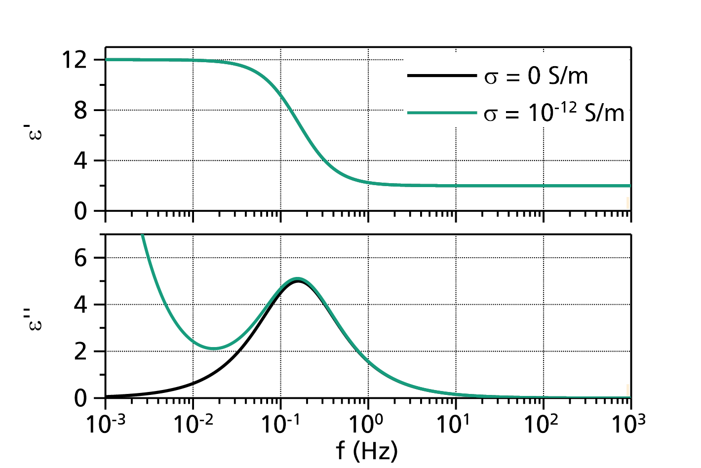
Fig. 2: Comparison of Havriliak-Negami (with ![]() ,
, ![]() ,
, ![]() ,
, ![]() and
and ![]() ) without and with DC conductivity. The values for
) without and with DC conductivity. The values for ![]() are indicated in the legend.
are indicated in the legend.
References:
Havriliak, S., Negami, S., "A complex plane representation of dielectric and mechanical relaxation processes in some polymers", Polymer 8: 161–210, doi:10.1016/0032-3861(67)90021-3
Havriliak-Negami retardation of the relative dielectric permittivity (circular frequency)
This function models the retardation of the relative dielectric permittivity in dependence on the circular frequency ![]() , including a term for the DC electric conductivity:
, including a term for the DC electric conductivity:
with ![]() being the complex relative dielectric permittivity of a material (the other quantities are described below).
It is a special case of the underlying base function with the options NumberOfTerms=1, UseFrequencyInsteadOfOmega=false, UseFlowTerm=true, IsRelativeDielectricPermittivity=true, InvertViscosity=true, InvertResult=false and LogarithmizeResult=false. These options can be changed by double-clicking on the fit function.
being the complex relative dielectric permittivity of a material (the other quantities are described below).
It is a special case of the underlying base function with the options NumberOfTerms=1, UseFrequencyInsteadOfOmega=false, UseFlowTerm=true, IsRelativeDielectricPermittivity=true, InvertViscosity=true, InvertResult=false and LogarithmizeResult=false. These options can be changed by double-clicking on the fit function.
The underlying base function models the generalized complex dynamic susceptibility in dependence on the frequency with one or more retardation terms and a flow term as:
with the circular frequency ![]() being the independent variable (or, depending on an option, the frequency
being the independent variable (or, depending on an option, the frequency ![]() ,
, ![]() ), and
), and ![]() and
and ![]() being the dependent variables, namely the real and negative imaginary part of the complex dynamic susceptibility
being the dependent variables, namely the real and negative imaginary part of the complex dynamic susceptibility ![]() .
.
Typical use cases are fits to the complex relative dielectric permittivity ![]() , to the complex mechanical compliance
, to the complex mechanical compliance ![]() , or the specific complex heat capacity
, or the specific complex heat capacity ![]() . With the option InvertResult=true, fits to the complex mechanical modulus
. With the option InvertResult=true, fits to the complex mechanical modulus ![]() or the dielectric modulus
or the dielectric modulus ![]() are possible, too.
are possible, too.
The parameters are:
- : high frequency susceptibility limit
- : retardation amplitude of term k
- : retardation time of term k
- , : shape exponents (usually and ) of term k
- : DC specific electrical conductivity in S/m
- : DC specific electrical resistance in Ω·m
- : generalized conductivity, for instance fluidity (inverse viscosity)
- : generalized viscosity
The available options are:
NumberOfTerms (
):
Determines the number of retardation terms in the formula above. Must be at least 1.
UseFrequencyInsteadOfOmega:
If true, the frequency is used as the independent variable, thus in the formula above is replaced by .
If false, the circular frequency () is used as the independent variable.
UseFlowTerm:
If true, the flow term in above formula is used.
If false, the flow term is not used, and the parameter corresponding with the flow term will not show in the fit.IsRelativeDielectricPermittivity:
If true, it is assumed that relative dielectric permittivity data are fitted. Thus, the flow term is modified to use either the DC specific electric conductivity or the DC specific electric resisitivity as the parameter for the flow term: or with being the vacuum permittivity..
InvertViscosity:
If true, the parameter in the flow term is an inverted viscosity (i.e. specific electrical conductivity, fluidity). Thus the flow term generally is.
If false, the parameter in the flow term is a viscosity, and the flow term generally is.
InvertResult:
If true, the result is inverted, i.e. instead of the general susceptibility the real and imaginary part of the generalized modulus is used for the dependent variables. Please note that despite the fact that the output is a modulus, the parameters are still retardation times (and not relaxation times)!
If false, the real and negative imaginary part of the generalized susceptibility are used as the dependent variables.LogarithmizeResult:
If true, the resulting values of and (or and if InvertResult is true) are logarithmized (decadic logarithm).
If false, the original values are used.
Note:
Since in some cases
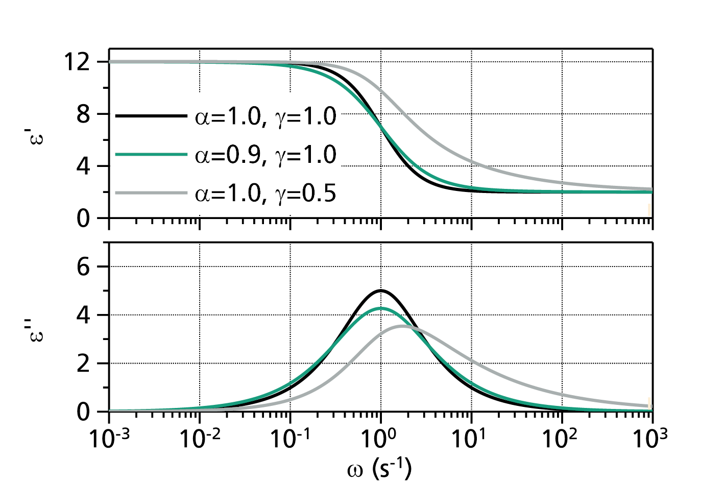
Fig. 1: Havriliak-Negami (with ![]() ,
, ![]() ,
, ![]() and
and ![]() ). The values for
). The values for ![]() and
and ![]() are indicated in the legend.
are indicated in the legend.
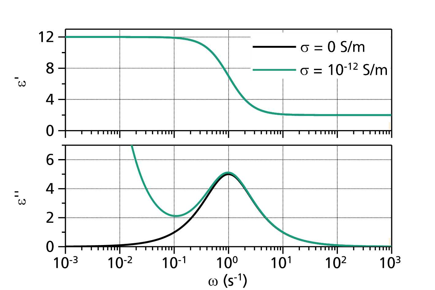
Fig. 2: Comparison of Havriliak-Negami (with ![]() ,
, ![]() ,
, ![]() ,
, ![]() and
and ![]() ) without and with DC conductivity. The values for
) without and with DC conductivity. The values for ![]() are indicated in the legend.
are indicated in the legend.
References:
Havriliak, S., Negami, S., "A complex plane representation of dielectric and mechanical relaxation processes in some polymers", Polymer 8: 161–210, doi:10.1016/0032-3861(67)90021-3
Kohlrausch retardation of the relative dielectric permittivity (frequency)
This function models the retardation of the relative dielectric permittivity in dependence on the frequency ![]() , including a term for the DC electric conductivity:
, including a term for the DC electric conductivity:

based on the Fourier transform of the derivative of the time-domain Kohlrausch function ![]() :
:
with ![]() being the complex relative dielectric permittivity of a material (the other quantities are described below).
It is a special case of the underlying base function with the options NumberOfTerms=1, UseFrequencyInsteadOfOmega=true, UseFlowTerm=true, IsRelativeDielectricPermittivity=true, InvertViscosity=true, InvertResult=false and LogarithmizeResult=false. These options can be changed by double-clicking on the fit function.
being the complex relative dielectric permittivity of a material (the other quantities are described below).
It is a special case of the underlying base function with the options NumberOfTerms=1, UseFrequencyInsteadOfOmega=true, UseFlowTerm=true, IsRelativeDielectricPermittivity=true, InvertViscosity=true, InvertResult=false and LogarithmizeResult=false. These options can be changed by double-clicking on the fit function.
The underlying base function models the generalized complex dynamic susceptibility in dependence on the frequency with one or more retardation terms and a flow term as:

based on the Fourier transformation of the time derivative of the Kohlrausch function ![]() , with the circular frequency
, with the circular frequency ![]() being the independent variable (or, depending on an option, the frequency
being the independent variable (or, depending on an option, the frequency ![]() ,
, ![]() ), and
), and ![]() and
and ![]() being the dependent variables, namely the real and negative imaginary part of the complex dynamic susceptibility
being the dependent variables, namely the real and negative imaginary part of the complex dynamic susceptibility ![]() .
.
Typical use cases are fits to the complex relative dielectric permittivity ![]() , to the complex mechanical compliance
, to the complex mechanical compliance ![]() , or the specific complex heat capacity
, or the specific complex heat capacity ![]() . With the option InvertResult=true, fits to the complex mechanical modulus
. With the option InvertResult=true, fits to the complex mechanical modulus ![]() or the dielectric modulus
or the dielectric modulus ![]() are possible, too.
are possible, too.
The parameters are:
- : high frequency susceptibility limit
- : retardation amplitude of term k
- : retardation time of term k
 : shape exponent (usually of term k
- : DC specific electrical conductivity in S/m
- : DC specific electrical resistance in Ω·m
- : generalized conductivity, for instance fluidity (inverse viscosity)
- : generalized viscosity
The available options are:
NumberOfTerms (
):
Determines the number of retardation terms in the formula above. Must be at least 1.
UseFrequencyInsteadOfOmega:
If true, the frequency is used as the independent variable, thus in the formula above is replaced by .
If false, the circular frequency () is used as the independent variable.
UseFlowTerm:
If true, the flow term in above formula is used.
If false, the flow term is not used, and the parameter corresponding with the flow term will not show in the fit.IsRelativeDielectricPermittivity:
If true, it is assumed that relative dielectric permittivity data are fitted. Thus, the flow term is modified to use either the DC specific electric conductivity or the DC specific electric resisitivity as the parameter for the flow term: or with being the vacuum permittivity..
InvertViscosity:
If true, the parameter in the flow term is an inverted viscosity (i.e. specific electrical conductivity, fluidity). Thus the flow term generally is.
If false, the parameter in the flow term is a viscosity, and the flow term generally is.
InvertResult:
If true, the result is inverted, i.e. instead of the general susceptibility the real and imaginary part of the generalized modulus is used for the dependent variables. Please note that despite the fact that the output is a modulus, the parameters are still retardation times (and not relaxation times)!
If false, the real and negative imaginary part of the generalized susceptibility are used as the dependent variables.LogarithmizeResult:
If true, the resulting values of and (or and if InvertResult is true) are logarithmized (decadic logarithm).
If false, the original values are used.
Note:
Since in some cases
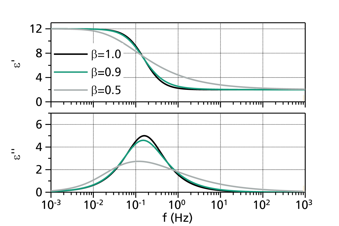
Fig. 1: Kohlrausch susceptibility fit functions (with ![]() ,
, ![]() ,
, ![]() and
and ![]() ). The values for
). The values for ![]() are indicated in the legend.
are indicated in the legend.
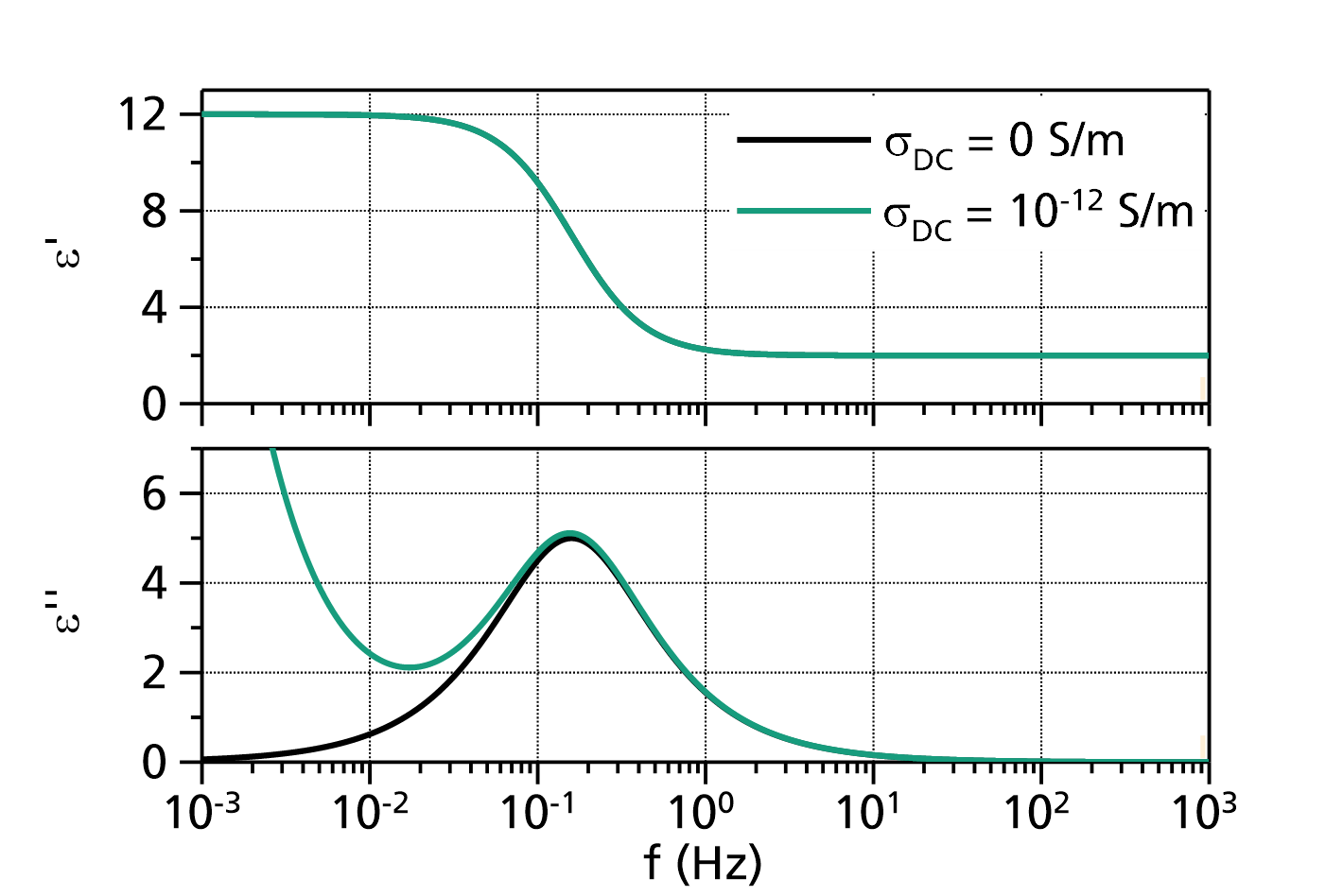
Fig. 2: Comparison of Kohlrausch susceptibility fit functions (with ![]() ,
, ![]() ,
, ![]() and
and ![]() ) without and with DC conductivity. The values for
) without and with DC conductivity. The values for ![]() are indicated in the legend.
are indicated in the legend.
References:
Kohlrausch, R., "Theorie des elektrischen Rückstandes in der Leidner Flasche", Annalen der Physik und Chemie. 91 (1) (1854): 56–82, 179–213, doi:10.1002/andp.18541670103
Williams, G., Watts, D. C., "Non-Symmetrical Dielectric Relaxation Behavior Arising from a Simple Empirical Decay Function", Transactions of the Faraday Society 66 (1970) 80–85. doi:10.1039/tf9706600080
Kohlrausch retardation of the relative dielectric permittivity (circular frequency)
This function models the retardation of the relative dielectric permittivity in dependence on the circular frequency ![]() , including a term for the DC electric conductivity:
, including a term for the DC electric conductivity:

based on the Fourier transform of the derivative of the time-domain Kohlrausch function ![]() :
:
with ![]() being the complex relative dielectric permittivity of a material (the other quantities are described below).
It is a special case of the underlying base function with the options NumberOfTerms=1, UseFrequencyInsteadOfOmega=false, UseFlowTerm=true, IsRelativeDielectricPermittivity=true, InvertViscosity=true, InvertResult=false and LogarithmizeResult=false. These options can be changed by double-clicking on the fit function.
being the complex relative dielectric permittivity of a material (the other quantities are described below).
It is a special case of the underlying base function with the options NumberOfTerms=1, UseFrequencyInsteadOfOmega=false, UseFlowTerm=true, IsRelativeDielectricPermittivity=true, InvertViscosity=true, InvertResult=false and LogarithmizeResult=false. These options can be changed by double-clicking on the fit function.
The underlying base function models the generalized complex dynamic susceptibility in dependence on the frequency with one or more retardation terms and a flow term as:
based on the Fourier transformation of the time derivative of the Kohlrausch function ![]() , with the circular frequency
, with the circular frequency ![]() being the independent variable (or, depending on an option, the frequency
being the independent variable (or, depending on an option, the frequency ![]() ,
, ![]() ), and
), and ![]() and
and ![]() being the dependent variables, namely the real and negative imaginary part of the complex dynamic susceptibility
being the dependent variables, namely the real and negative imaginary part of the complex dynamic susceptibility ![]() .
.
Typical use cases are fits to the complex relative dielectric permittivity ![]() , to the complex mechanical compliance
, to the complex mechanical compliance ![]() , or the specific complex heat capacity
, or the specific complex heat capacity ![]() . With the option InvertResult=true, fits to the complex mechanical modulus
. With the option InvertResult=true, fits to the complex mechanical modulus ![]() or the dielectric modulus
or the dielectric modulus ![]() are possible, too.
are possible, too.
The parameters are:
- : high frequency susceptibility limit
- : retardation amplitude of term k
- : retardation time of term k
- : shape exponent (usually of term k
- : DC specific electrical conductivity in S/m
- : DC specific electrical resistance in Ω·m
- : generalized conductivity, for instance fluidity (inverse viscosity)
- : generalized viscosity
The available options are:
NumberOfTerms (
):
Determines the number of retardation terms in the formula above. Must be at least 1.
UseFrequencyInsteadOfOmega:
If true, the frequency is used as the independent variable, thus in the formula above is replaced by .
If false, the circular frequency () is used as the independent variable.
UseFlowTerm:
If true, the flow term in above formula is used.
If false, the flow term is not used, and the parameter corresponding with the flow term will not show in the fit.IsRelativeDielectricPermittivity:
If true, it is assumed that relative dielectric permittivity data are fitted. Thus, the flow term is modified to use either the DC specific electric conductivity or the DC specific electric resisitivity as the parameter for the flow term: or with being the vacuum permittivity..
InvertViscosity:
If true, the parameter in the flow term is an inverted viscosity (i.e. specific electrical conductivity, fluidity). Thus the flow term generally is.
If false, the parameter in the flow term is a viscosity, and the flow term generally is.
InvertResult:
If true, the result is inverted, i.e. instead of the general susceptibility the real and imaginary part of the generalized modulus is used for the dependent variables. Please note that despite the fact that the output is a modulus, the parameters are still retardation times (and not relaxation times)!
If false, the real and negative imaginary part of the generalized susceptibility are used as the dependent variables.LogarithmizeResult:
If true, the resulting values of and (or and if InvertResult is true) are logarithmized (decadic logarithm).
If false, the original values are used.
Note:
Since in some cases
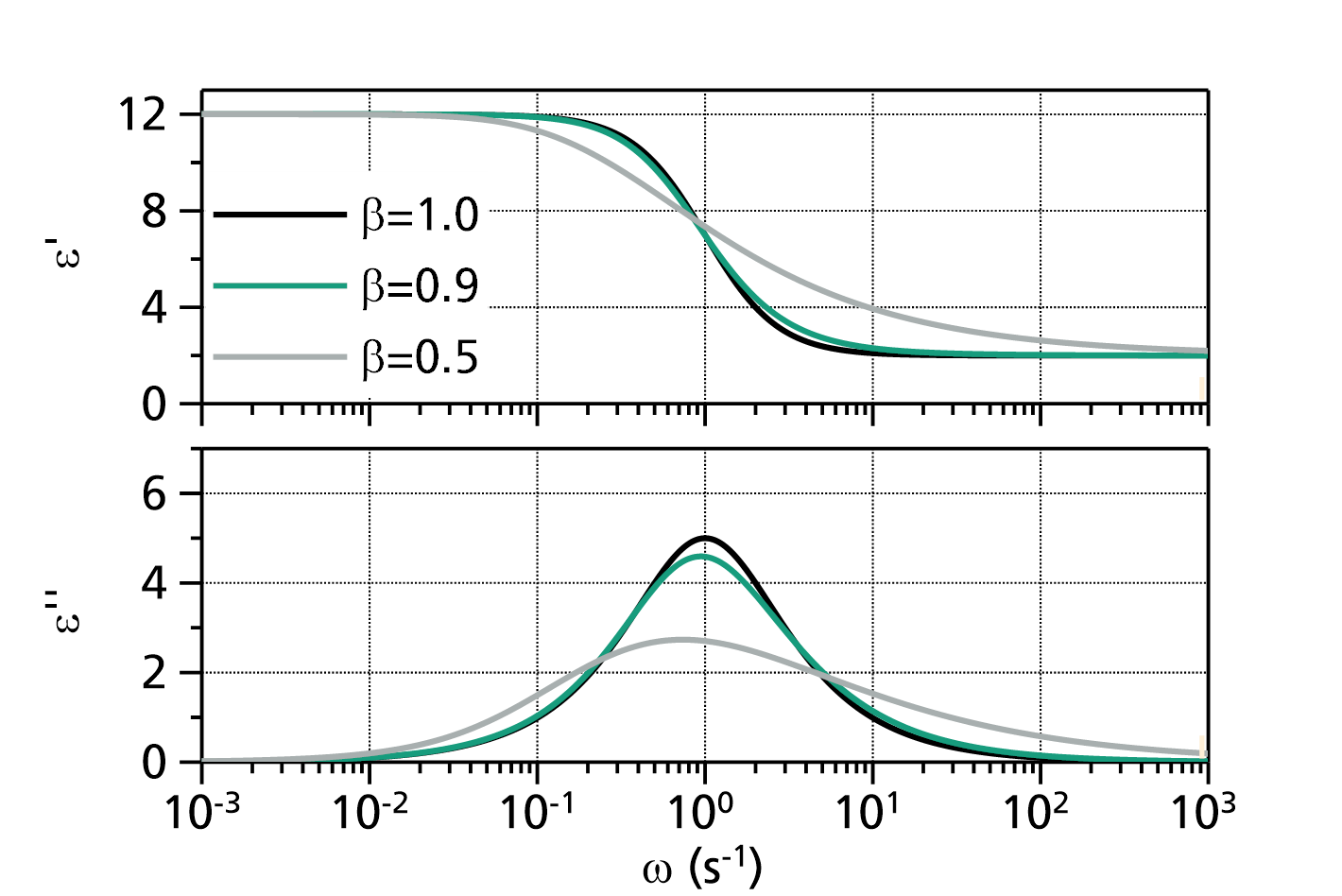
Fig. 1: Kohlrausch susceptibility fit functions (with ![]() ,
, ![]() ,
, ![]() and
and ![]() ). The values for
). The values for ![]() are indicated in the legend.
are indicated in the legend.
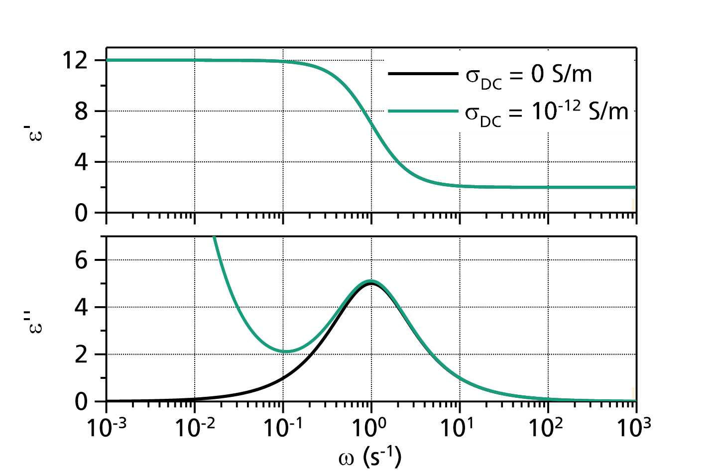
Fig. 2: Comparison of Kohlrausch susceptibility fit functions (with ![]() ,
, ![]() ,
, ![]() and
and ![]() ) without and with DC conductivity. The values for
) without and with DC conductivity. The values for ![]() are indicated in the legend.
are indicated in the legend.
References:
Kohlrausch, R., "Theorie des elektrischen Rückstandes in der Leidner Flasche", Annalen der Physik und Chemie. 91 (1) (1854): 56–82, 179–213, doi:10.1002/andp.18541670103
Williams, G., Watts, D. C., "Non-Symmetrical Dielectric Relaxation Behavior Arising from a Simple Empirical Decay Function", Transactions of the Faraday Society 66 (1970) 80–85. doi:10.1039/tf9706600080
General retardation fit functions
Havriliak-Negami retardation of a general susceptibility (frequency)
This function models the retardation of a general susceptibility (e.g. mechanical complicance) in dependence on the frequency ![]() , including a term for the flow:
, including a term for the flow:
The quantities are described below. It is a special case of the underlying base function with the options NumberOfTerms=1, UseFrequencyInsteadOfOmega=true, UseFlowTerm=true, IsRelativeDielectricPermittivity=false, InvertViscosity=false, InvertResult=false and LogarithmizeResult=false. These options can be changed by double-clicking on the fit function.
The underlying base function models the generalized complex dynamic susceptibility in dependence on the frequency with one or more retardation terms and a flow term as:
with the circular frequency ![]() being the independent variable (or, depending on an option, the frequency
being the independent variable (or, depending on an option, the frequency ![]() ,
, ![]() ), and
), and ![]() and
and ![]() being the dependent variables, namely the real and negative imaginary part of the complex dynamic susceptibility
being the dependent variables, namely the real and negative imaginary part of the complex dynamic susceptibility ![]() .
.
Typical use cases are fits to the complex relative dielectric permittivity ![]() , to the complex mechanical compliance
, to the complex mechanical compliance ![]() , or the specific complex heat capacity
, or the specific complex heat capacity ![]() . With the option InvertResult=true, fits to the complex mechanical modulus
. With the option InvertResult=true, fits to the complex mechanical modulus ![]() or the dielectric modulus
or the dielectric modulus ![]() are possible, too.
are possible, too.
The parameters are:
- : high frequency susceptibility limit
- : retardation amplitude of term k
- : retardation time of term k
- , : shape exponents (usually and ) of term k
- : DC specific electrical conductivity in S/m
- : DC specific electrical resistance in Ω·m
- : generalized conductivity, for instance fluidity (inverse viscosity)
- : generalized viscosity
The available options are:
NumberOfTerms (
):
Determines the number of retardation terms in the formula above. Must be at least 1.
UseFrequencyInsteadOfOmega:
If true, the frequency is used as the independent variable, thus in the formula above is replaced by .
If false, the circular frequency () is used as the independent variable.
UseFlowTerm:
If true, the flow term in above formula is used.
If false, the flow term is not used, and the parameter corresponding with the flow term will not show in the fit.IsRelativeDielectricPermittivity:
If true, it is assumed that relative dielectric permittivity data are fitted. Thus, the flow term is modified to use either the DC specific electric conductivity or the DC specific electric resisitivity as the parameter for the flow term: or with being the vacuum permittivity..
InvertViscosity:
If true, the parameter in the flow term is an inverted viscosity (i.e. specific electrical conductivity, fluidity). Thus the flow term generally is.
If false, the parameter in the flow term is a viscosity, and the flow term generally is.
InvertResult:
If true, the result is inverted, i.e. instead of the general susceptibility the real and imaginary part of the generalized modulus is used for the dependent variables. Please note that despite the fact that the output is a modulus, the parameters are still retardation times (and not relaxation times)!
If false, the real and negative imaginary part of the generalized susceptibility are used as the dependent variables.LogarithmizeResult:
If true, the resulting values of and (or and if InvertResult is true) are logarithmized (decadic logarithm).
If false, the original values are used.
Note:
Since in some cases
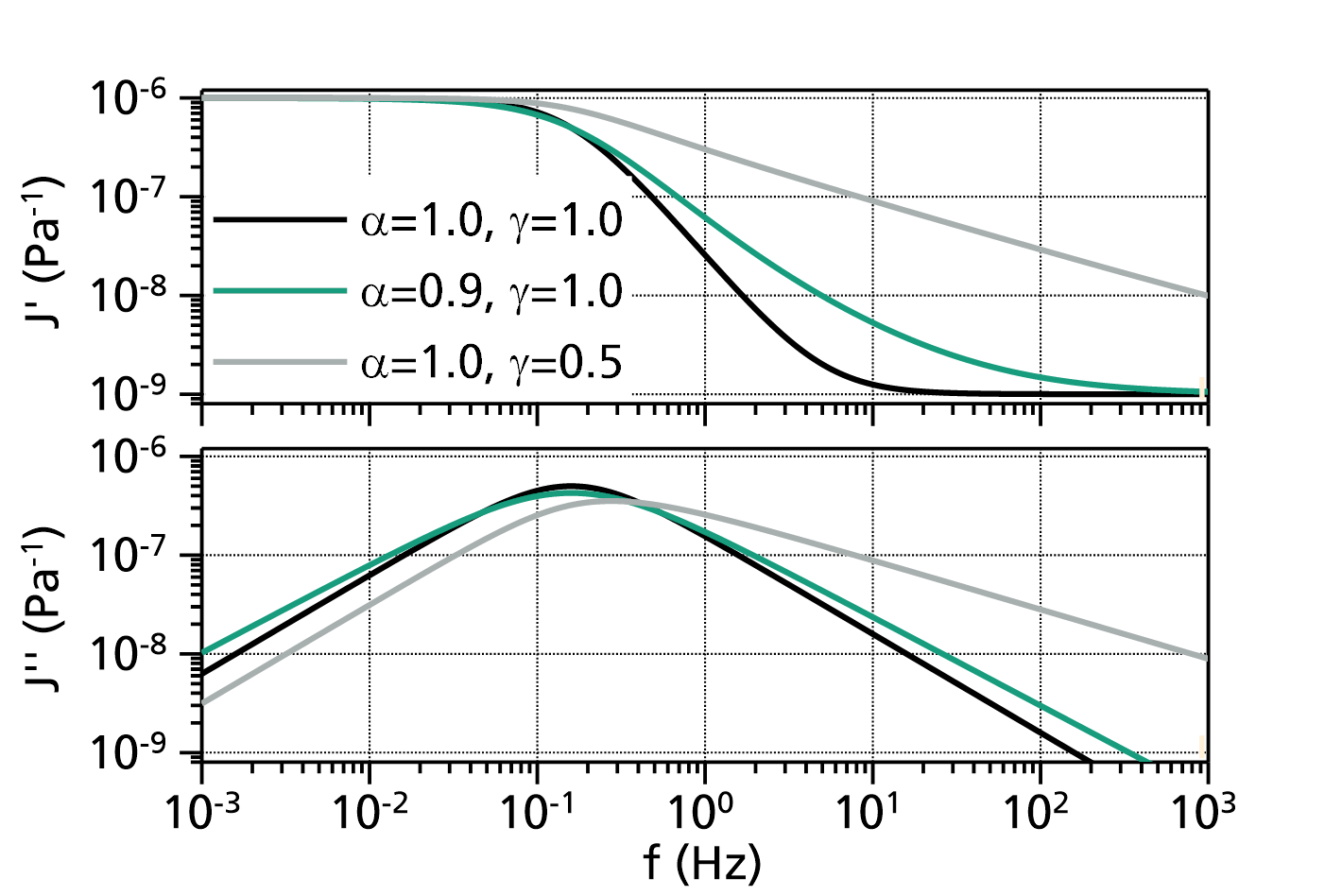
Fig. 1: Havriliak-Negami (with ![]() ,
, ![]() ,
, ![]() and
and ![]() ). The values for
). The values for ![]() and
and ![]() are indicated in the legend.
are indicated in the legend.
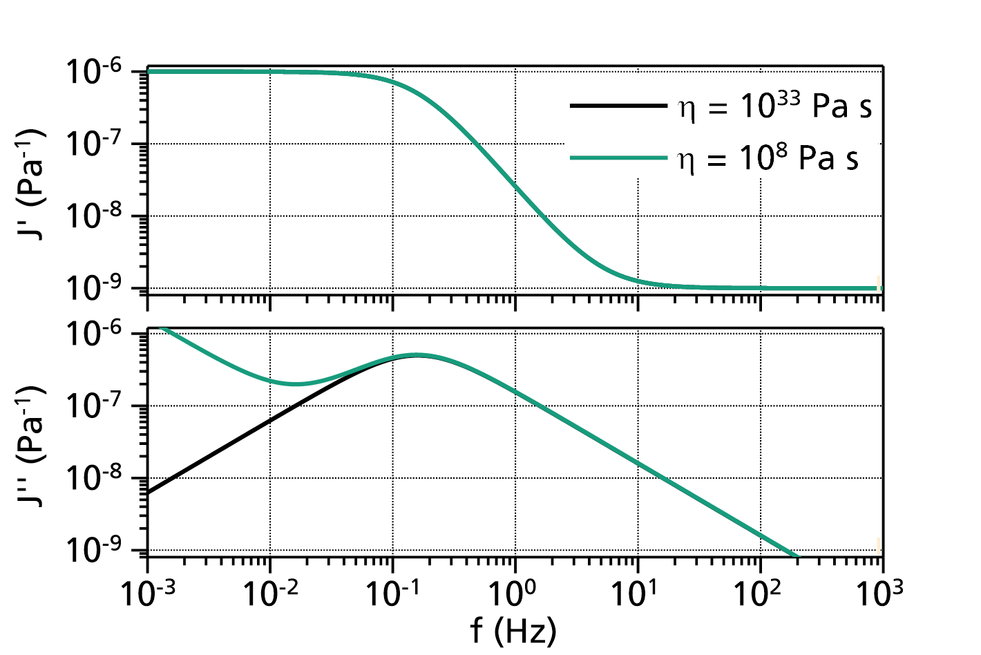
Fig. 2: Comparison of Havriliak-Negami (with ![]() ,
, ![]() ,
, ![]() ,
, ![]() and
and ![]() ) with different viscosities
) with different viscosities ![]() . The values for
. The values for ![]() are indicated in the legend.
are indicated in the legend.
References:
Havriliak, S., Negami, S., "A complex plane representation of dielectric and mechanical relaxation processes in some polymers", Polymer 8: 161–210, doi:10.1016/0032-3861(67)90021-3
Havriliak-Negami retardation of a general susceptibility (circular frequency)
This function models the retardation of a general susceptibility (e.g. mechanical complicance) in dependence on the circular frequency ![]() , including a term for the flow:
, including a term for the flow:
The quantities are described below. It is a special case of the underlying base function with the options NumberOfTerms=1, UseFrequencyInsteadOfOmega=false, UseFlowTerm=true, IsRelativeDielectricPermittivity=false, InvertViscosity=false, InvertResult=false and LogarithmizeResult=false. These options can be changed by double-clicking on the fit function.
The underlying base function models the generalized complex dynamic susceptibility in dependence on the frequency with one or more retardation terms and a flow term as:
with the circular frequency ![]() being the independent variable (or, depending on an option, the frequency
being the independent variable (or, depending on an option, the frequency ![]() ,
, ![]() ), and
), and ![]() and
and ![]() being the dependent variables, namely the real and negative imaginary part of the complex dynamic susceptibility
being the dependent variables, namely the real and negative imaginary part of the complex dynamic susceptibility ![]() .
.
Typical use cases are fits to the complex relative dielectric permittivity ![]() , to the complex mechanical compliance
, to the complex mechanical compliance ![]() , or the specific complex heat capacity
, or the specific complex heat capacity ![]() . With the option InvertResult=true, fits to the complex mechanical modulus
. With the option InvertResult=true, fits to the complex mechanical modulus ![]() or the dielectric modulus
or the dielectric modulus ![]() are possible, too.
are possible, too.
The parameters are:
- : high frequency susceptibility limit
- : retardation amplitude of term k
- : retardation time of term k
- , : shape exponents (usually and ) of term k
- : DC specific electrical conductivity in S/m
- : DC specific electrical resistance in Ω·m
- : generalized conductivity, for instance fluidity (inverse viscosity)
- : generalized viscosity
The available options are:
NumberOfTerms (
):
Determines the number of retardation terms in the formula above. Must be at least 1.
UseFrequencyInsteadOfOmega:
If true, the frequency is used as the independent variable, thus in the formula above is replaced by .
If false, the circular frequency () is used as the independent variable.
UseFlowTerm:
If true, the flow term in above formula is used.
If false, the flow term is not used, and the parameter corresponding with the flow term will not show in the fit.IsRelativeDielectricPermittivity:
If true, it is assumed that relative dielectric permittivity data are fitted. Thus, the flow term is modified to use either the DC specific electric conductivity or the DC specific electric resisitivity as the parameter for the flow term: or with being the vacuum permittivity..
InvertViscosity:
If true, the parameter in the flow term is an inverted viscosity (i.e. specific electrical conductivity, fluidity). Thus the flow term generally is.
If false, the parameter in the flow term is a viscosity, and the flow term generally is.
InvertResult:
If true, the result is inverted, i.e. instead of the general susceptibility the real and imaginary part of the generalized modulus is used for the dependent variables. Please note that despite the fact that the output is a modulus, the parameters are still retardation times (and not relaxation times)!
If false, the real and negative imaginary part of the generalized susceptibility are used as the dependent variables.LogarithmizeResult:
If true, the resulting values of and (or and if InvertResult is true) are logarithmized (decadic logarithm).
If false, the original values are used.
Note:
Since in some cases
Fig. 1: Havriliak-Negami (with ![]() ,
, ![]() ,
, ![]() and
and ![]() ). The values for
). The values for ![]() and
and ![]() are indicated in the legend.
are indicated in the legend.

Fig. 2: Comparison of Havriliak-Negami (with ![]() ,
, ![]() ,
, ![]() ,
, ![]() and
and ![]() ) with different viscosities
) with different viscosities ![]() . The values for
. The values for ![]() are indicated in the legend.
are indicated in the legend.
References:
Havriliak, S., Negami, S., "A complex plane representation of dielectric and mechanical relaxation processes in some polymers", Polymer 8: 161–210, doi:10.1016/0032-3861(67)90021-3
Kohlrausch retardation of a general susceptibility (frequency)
This function models the retardation of a general susceptibility (e.g. mechanical complicance) in dependence on the frequency ![]() , including a term for the flow:
, including a term for the flow:

based on the Fourier transform of the derivative of the time-domain Kohlrausch function ![]() :
:
The quantities are described below. It is a special case of the underlying base function with the options NumberOfTerms=1, UseFrequencyInsteadOfOmega=true, UseFlowTerm=true, IsRelativeDielectricPermittivity=false, InvertViscosity=false, InvertResult=false and LogarithmizeResult=false. These options can be changed by double-clicking on the fit function.
The underlying base function models the generalized complex dynamic susceptibility in dependence on the frequency with one or more retardation terms and a flow term as:
based on the Fourier transformation of the time derivative of the Kohlrausch function ![]() , with the circular frequency
, with the circular frequency ![]() being the independent variable (or, depending on an option, the frequency
being the independent variable (or, depending on an option, the frequency ![]() ,
, ![]() ), and
), and ![]() and
and ![]() being the dependent variables, namely the real and negative imaginary part of the complex dynamic susceptibility
being the dependent variables, namely the real and negative imaginary part of the complex dynamic susceptibility ![]() .
.
Typical use cases are fits to the complex relative dielectric permittivity ![]() , to the complex mechanical compliance
, to the complex mechanical compliance ![]() , or the specific complex heat capacity
, or the specific complex heat capacity ![]() . With the option InvertResult=true, fits to the complex mechanical modulus
. With the option InvertResult=true, fits to the complex mechanical modulus ![]() or the dielectric modulus
or the dielectric modulus ![]() are possible, too.
are possible, too.
The parameters are:
- : high frequency susceptibility limit
- : retardation amplitude of term k
- : retardation time of term k
- : shape exponent (usually of term k
- : DC specific electrical conductivity in S/m
- : DC specific electrical resistance in Ω·m
- : generalized conductivity, for instance fluidity (inverse viscosity)
- : generalized viscosity
The available options are:
NumberOfTerms (
):
Determines the number of retardation terms in the formula above. Must be at least 1.
UseFrequencyInsteadOfOmega:
If true, the frequency is used as the independent variable, thus in the formula above is replaced by .
If false, the circular frequency () is used as the independent variable.
UseFlowTerm:
If true, the flow term in above formula is used.
If false, the flow term is not used, and the parameter corresponding with the flow term will not show in the fit.IsRelativeDielectricPermittivity:
If true, it is assumed that relative dielectric permittivity data are fitted. Thus, the flow term is modified to use either the DC specific electric conductivity or the DC specific electric resisitivity as the parameter for the flow term: or with being the vacuum permittivity..
InvertViscosity:
If true, the parameter in the flow term is an inverted viscosity (i.e. specific electrical conductivity, fluidity). Thus the flow term generally is.
If false, the parameter in the flow term is a viscosity, and the flow term generally is.
InvertResult:
If true, the result is inverted, i.e. instead of the general susceptibility the real and imaginary part of the generalized modulus is used for the dependent variables. Please note that despite the fact that the output is a modulus, the parameters are still retardation times (and not relaxation times)!
If false, the real and negative imaginary part of the generalized susceptibility are used as the dependent variables.LogarithmizeResult:
If true, the resulting values of and (or and if InvertResult is true) are logarithmized (decadic logarithm).
If false, the original values are used.
Note:
Since in some cases
Fig. 1: Kohlrausch susceptibility fit functions (with ![]() ,
, ![]() ,
, ![]() and
and ![]() ). The values for
). The values for ![]() are indicated in the legend.
are indicated in the legend.
Fig. 2: Comparison of Kohlrausch susceptibility fit functions (with ![]() ,
, ![]() ,
, ![]() and
and ![]() ) with different viscosities
) with different viscosities ![]() . The values for
. The values for ![]() are indicated in the legend.
are indicated in the legend.
References:
Kohlrausch, R., "Theorie des elektrischen Rückstandes in der Leidner Flasche", Annalen der Physik und Chemie. 91 (1) (1854): 56–82, 179–213, doi:10.1002/andp.18541670103
Williams, G., Watts, D. C., "Non-Symmetrical Dielectric Relaxation Behavior Arising from a Simple Empirical Decay Function", Transactions of the Faraday Society 66 (1970) 80–85. doi:10.1039/tf9706600080
Kohlrausch retardation of a general susceptibility (circular frequency)
This function models the retardation of a general susceptibility (e.g. mechanical complicance) in dependence on the circular frequency ![]() , including a term for the flow:
, including a term for the flow:

based on the Fourier transform of the derivative of the time-domain Kohlrausch function ![]() .
.
The quantities are described below. It is a special case of the underlying base function with the options NumberOfTerms=1, UseFrequencyInsteadOfOmega=false, UseFlowTerm=true, IsRelativeDielectricPermittivity=false, InvertViscosity=false, InvertResult=false and LogarithmizeResult=false. These options can be changed by double-clicking on the fit function.
The underlying base function models the generalized complex dynamic susceptibility in dependence on the frequency with one or more retardation terms and a flow term as:
based on the Fourier transformation of the time derivative of the Kohlrausch function ![]() , with the circular frequency
, with the circular frequency ![]() being the independent variable (or, depending on an option, the frequency
being the independent variable (or, depending on an option, the frequency ![]() ,
, ![]() ), and
), and ![]() and
and ![]() being the dependent variables, namely the real and negative imaginary part of the complex dynamic susceptibility
being the dependent variables, namely the real and negative imaginary part of the complex dynamic susceptibility ![]() .
.
Typical use cases are fits to the complex relative dielectric permittivity ![]() , to the complex mechanical compliance
, to the complex mechanical compliance ![]() , or the specific complex heat capacity
, or the specific complex heat capacity ![]() . With the option InvertResult=true, fits to the complex mechanical modulus
. With the option InvertResult=true, fits to the complex mechanical modulus ![]() or the dielectric modulus
or the dielectric modulus ![]() are possible, too.
are possible, too.
The parameters are:
- : high frequency susceptibility limit
- : retardation amplitude of term k
- : retardation time of term k
- : shape exponent (usually of term k
- : DC specific electrical conductivity in S/m
- : DC specific electrical resistance in Ω·m
- : generalized conductivity, for instance fluidity (inverse viscosity)
- : generalized viscosity
The available options are:
NumberOfTerms (
):
Determines the number of retardation terms in the formula above. Must be at least 1.
UseFrequencyInsteadOfOmega:
If true, the frequency is used as the independent variable, thus in the formula above is replaced by .
If false, the circular frequency () is used as the independent variable.
UseFlowTerm:
If true, the flow term in above formula is used.
If false, the flow term is not used, and the parameter corresponding with the flow term will not show in the fit.IsRelativeDielectricPermittivity:
If true, it is assumed that relative dielectric permittivity data are fitted. Thus, the flow term is modified to use either the DC specific electric conductivity or the DC specific electric resisitivity as the parameter for the flow term: or with being the vacuum permittivity..
InvertViscosity:
If true, the parameter in the flow term is an inverted viscosity (i.e. specific electrical conductivity, fluidity). Thus the flow term generally is.
If false, the parameter in the flow term is a viscosity, and the flow term generally is.
InvertResult:
If true, the result is inverted, i.e. instead of the general susceptibility the real and imaginary part of the generalized modulus is used for the dependent variables. Please note that despite the fact that the output is a modulus, the parameters are still retardation times (and not relaxation times)!
If false, the real and negative imaginary part of the generalized susceptibility are used as the dependent variables.LogarithmizeResult:
If true, the resulting values of and (or and if InvertResult is true) are logarithmized (decadic logarithm).
If false, the original values are used.
Note:
Since in some cases
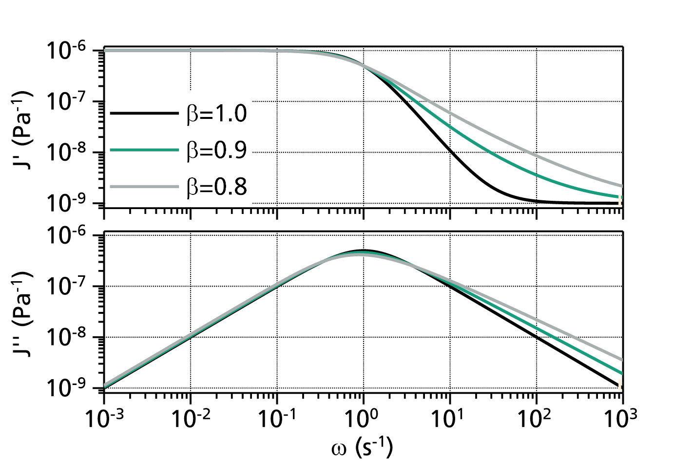
Fig. 1: Kohlrausch susceptibility fit functions (with ![]() ,
, ![]() ,
, ![]() and
and ![]() ). The values for
). The values for ![]() are indicated in the legend.
are indicated in the legend.
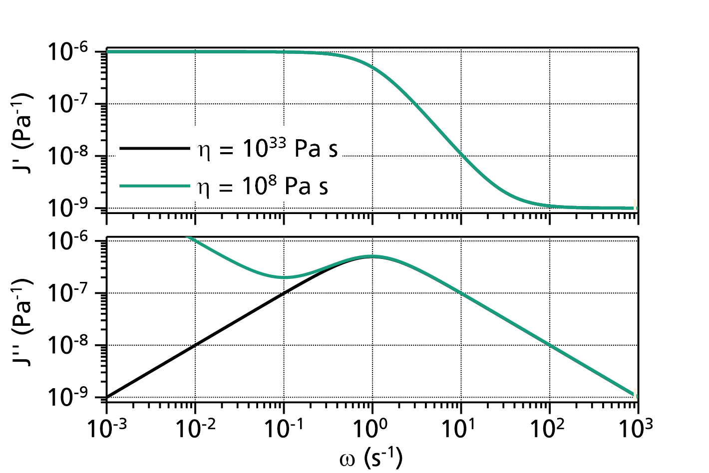
Fig. 2: Comparison of Kohlrausch susceptibility fit functions (with ![]() ,
, ![]() ,
, ![]() and
and ![]() ) with different viscosities
) with different viscosities ![]() . The values for
. The values for ![]() are indicated in the legend.
are indicated in the legend.
References:
Kohlrausch, R., "Theorie des elektrischen Rückstandes in der Leidner Flasche", Annalen der Physik und Chemie. 91 (1) (1854): 56–82, 179–213, doi:10.1002/andp.18541670103
Williams, G., Watts, D. C., "Non-Symmetrical Dielectric Relaxation Behavior Arising from a Simple Empirical Decay Function", Transactions of the Faraday Society 66 (1970) 80–85. doi:10.1039/tf9706600080
Modulus retardation fit functions
Note:
The quantity modulus generally corresponds with relaxation, not retardation! Therefore the fit functions in this folder primarily model susceptibility, which is afterwards converted into a modulus (by inverting the complex value).
Havriliak-Negami retardation of a general modulus (frequency)
This function models the retardation of a general modulus (e.g. mechanical modulus) in dependence on the frequency ![]() with a retardation and a flow term:
with a retardation and a flow term:
The quantities are described below. It is a special case of the underlying base function with the options UseFrequencyInsteadOfOmega=true, UseFlowTerm=true, InvertViscosity=false and LogarithmizeResult=false. These options can be changed by double-clicking on the fit function.
The underlying base function models the generalized complex dynamic modulus in dependence on the circular frequency ![]() as:
as:

with the circular frequency ![]() being the independent variable (or, depending on an option, the frequency
being the independent variable (or, depending on an option, the frequency ![]() ,
, ![]() ), and
), and ![]() and
and ![]() being the dependent variables, namely the real and imaginary part of the complex dynamic modulus
being the dependent variables, namely the real and imaginary part of the complex dynamic modulus ![]() .
.
The typical use case is a fit to the complex dynamic mechanical modulus (e.g. shear modulus ![]() or Young's modulus
or Young's modulus ![]() ).
).
The parameters are:
- : high frequency modulus limit
- : low frequency modulus limit
- : retardation time (attention: this is not the same as the relaxation time, e.g. the maximum of is considerably shifted with respect to
 !)
!)
- , : shape exponents (usually and )
- : generalized fluidity (inverse viscosity)
- : generalized viscosity
The available options are:
UseFrequencyInsteadOfOmega:
If true, the frequency is used as the independent variable, thus in the formula above is replaced by .
If false, the circular frequency is used as the independent variable.
UseFlowTerm:
If true, the flow term in above formula is used.
If false, the flow term is not used, and the parameter corresponding with the flow term will not show in the fit.InvertViscosity:
If true, the parameter in the flow term is an inverted viscosity (i.e. fluidity). Thus the flow term generally is.
If false, the parameter in the flow term is a viscosity, and the flow term generally is.
LogarithmizeResult:
If true, the resulting values of and are logarithmized (decadic logarithm).
If false, the original values are used.
Note:
Since in most cases
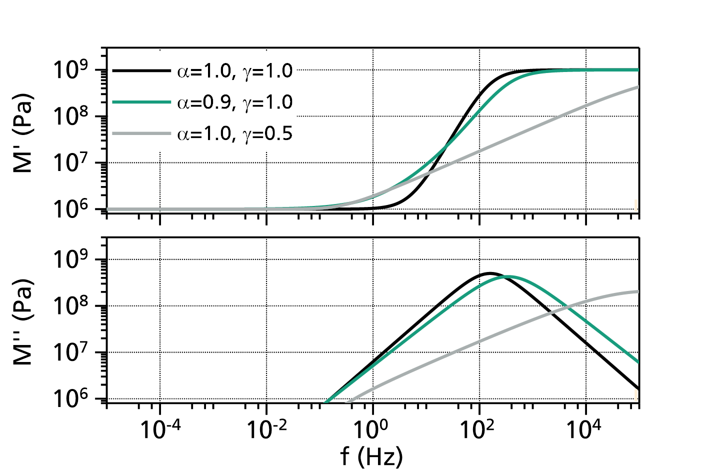
Fig. 1: Havriliak-Negami fit functions (with ![]() ,
, ![]() ,
, ![]() and
and ![]() ). The values for
). The values for ![]() and
and ![]() are indicated in the legend.
are indicated in the legend.
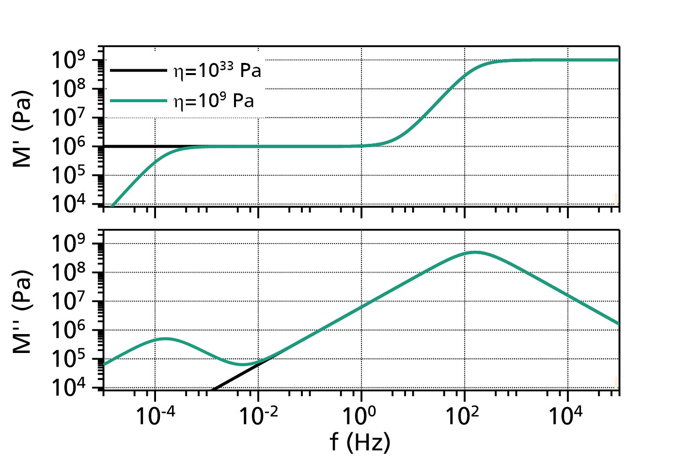
Fig. 2: Comparison of Havriliak-Negami fit functions (with ![]() ,
, ![]() ,
, ![]() ,
, ![]() and
and ![]() ) with different viscosities
) with different viscosities ![]() . The values for
. The values for ![]() are indicated in the legend.
are indicated in the legend.
References:
Havriliak, S., Negami, S., "A complex plane representation of dielectric and mechanical relaxation processes in some polymers", Polymer 8: 161–210, doi:10.1016/0032-3861(67)90021-3
Havriliak-Negami retardation of a general modulus (circular frequency)
This function models the retardation of a general modulus (e.g. mechanical modulus) in dependence on the circular frequency ![]() with a retardation and a flow term:
with a retardation and a flow term:
The quantities are described below. It is a special case of the underlying base function with the options UseFrequencyInsteadOfOmega=false, UseFlowTerm=true, InvertViscosity=false and LogarithmizeResult=false. These options can be changed by double-clicking on the fit function.
The underlying base function models the generalized complex dynamic modulus in dependence on the circular frequency ![]() as:
as:
with the circular frequency ![]() being the independent variable (or, depending on an option, the frequency
being the independent variable (or, depending on an option, the frequency ![]() ,
, ![]() ), and
), and ![]() and
and ![]() being the dependent variables, namely the real and imaginary part of the complex dynamic modulus
being the dependent variables, namely the real and imaginary part of the complex dynamic modulus ![]() .
.
The typical use case is a fit to the complex dynamic mechanical modulus (e.g. shear modulus ![]() or Young's modulus
or Young's modulus ![]() ).
).
The parameters are:
- : high frequency modulus limit
- : low frequency modulus limit
- : retardation time (attention: this is not the same as the relaxation time, e.g. the maximum of is considerably shifted with respect to !)
- , : shape exponents (usually and )
- : generalized fluidity (inverse viscosity)
- : generalized viscosity
The available options are:
UseFrequencyInsteadOfOmega:
If true, the frequency is used as the independent variable, thus in the formula above is replaced by .
If false, the circular frequency is used as the independent variable.
UseFlowTerm:
If true, the flow term in above formula is used.
If false, the flow term is not used, and the parameter corresponding with the flow term will not show in the fit.InvertViscosity:
If true, the parameter in the flow term is an inverted viscosity (i.e. fluidity). Thus the flow term generally is.
If false, the parameter in the flow term is a viscosity, and the flow term generally is.
LogarithmizeResult:
If true, the resulting values of and are logarithmized (decadic logarithm).
If false, the original values are used.
Note:
Since in most cases
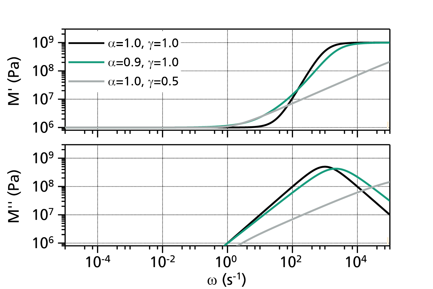
Fig. 1: Havriliak-Negami fit functions (with ![]() ,
, ![]() ,
, ![]() and
and ![]() ). The values for
). The values for ![]() and
and ![]() are indicated in the legend.
are indicated in the legend.
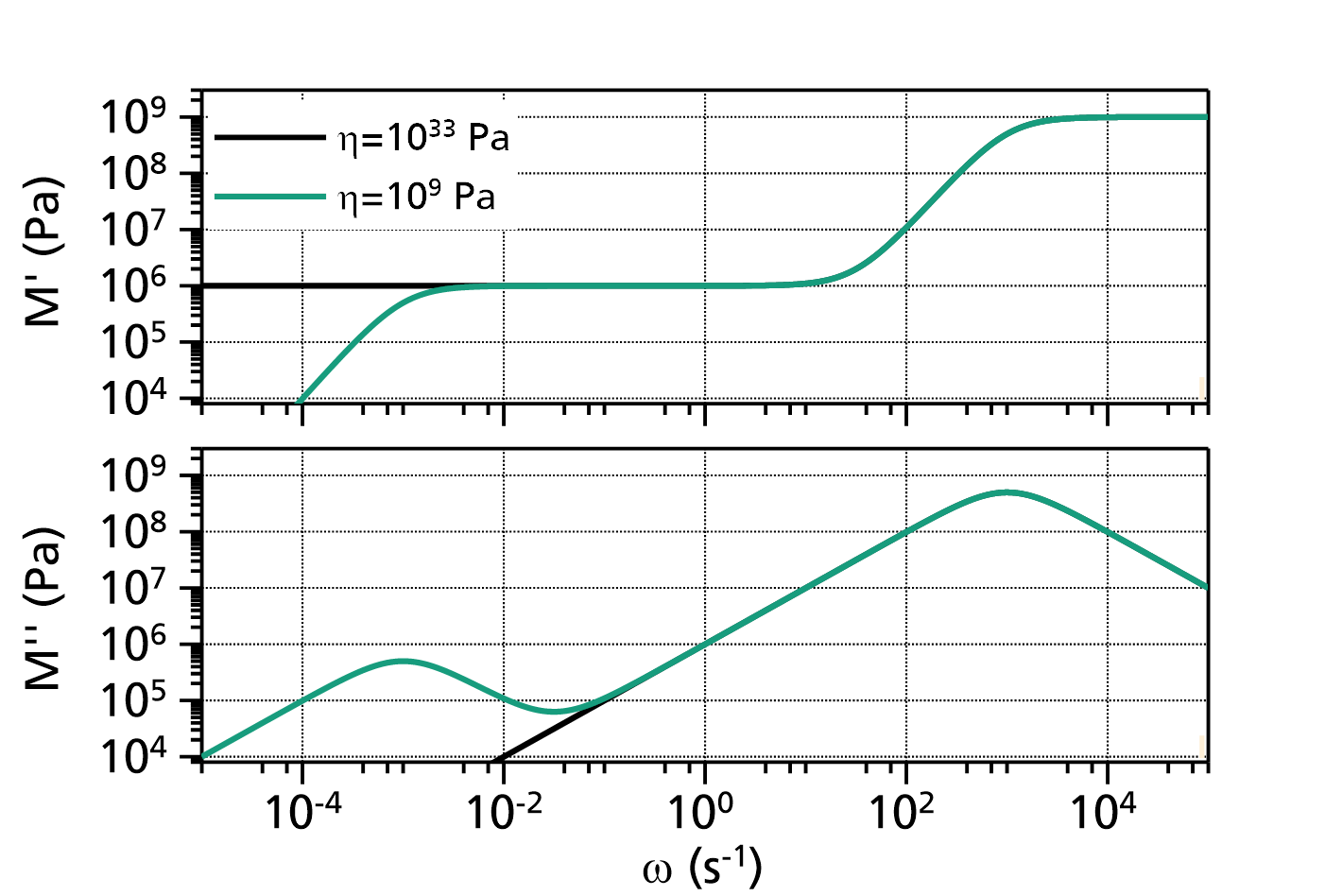
Fig. 2: Comparison of Havriliak-Negami fit functions (with ![]() ,
, ![]() ,
, ![]() ,
, ![]() and
and ![]() ) with different viscosities
) with different viscosities ![]() . The values for
. The values for ![]() are indicated in the legend.
are indicated in the legend.
References:
Havriliak, S., Negami, S., "A complex plane representation of dielectric and mechanical relaxation processes in some polymers", Polymer 8: 161–210, doi:10.1016/0032-3861(67)90021-3
Havriliak-Negami retardation of a general modulus (frequency)
This function models the retardation of a general modulus (e.g. mechanical modulus) in dependence on the frequency ![]() with two retardation terms and a term for the flow:
with two retardation terms and a term for the flow:
The quantities are described below. It is a special case of the underlying base function with the options NumberOfTerms=2, UseFrequencyInsteadOfOmega=true, UseFlowTerm=true, IsRelativeDielectricPermittivity=false, InvertViscosity=false, InvertResult=true and LogarithmizeResult=false. These options can be changed by double-clicking on the fit function.
The underlying base function models the generalized complex dynamic susceptibility in dependence on the frequency with one or more retardation terms and a flow term as:
with the circular frequency ![]() being the independent variable (or, depending on an option, the frequency
being the independent variable (or, depending on an option, the frequency ![]() ,
, ![]() ), and
), and ![]() and
and ![]() being the dependent variables, namely the real and negative imaginary part of the complex dynamic susceptibility
being the dependent variables, namely the real and negative imaginary part of the complex dynamic susceptibility ![]() .
.
Typical use cases are fits to the complex relative dielectric permittivity ![]() , to the complex mechanical compliance
, to the complex mechanical compliance ![]() , or the specific complex heat capacity
, or the specific complex heat capacity ![]() . With the option InvertResult=true, fits to the complex mechanical modulus
. With the option InvertResult=true, fits to the complex mechanical modulus ![]() or the dielectric modulus
or the dielectric modulus ![]() are possible, too.
are possible, too.
The parameters are:
- : high frequency susceptibility limit
- : retardation amplitude of term k
- : retardation time of term k
- , : shape exponents (usually and ) of term k
- : DC specific electrical conductivity in S/m
- : DC specific electrical resistance in Ω·m
- : generalized conductivity, for instance fluidity (inverse viscosity)
- : generalized viscosity
The available options are:
NumberOfTerms (
):
Determines the number of retardation terms in the formula above. Must be at least 1.
UseFrequencyInsteadOfOmega:
If true, the frequency is used as the independent variable, thus in the formula above is replaced by .
If false, the circular frequency () is used as the independent variable.
UseFlowTerm:
If true, the flow term in above formula is used.
If false, the flow term is not used, and the parameter corresponding with the flow term will not show in the fit.IsRelativeDielectricPermittivity:
If true, it is assumed that relative dielectric permittivity data are fitted. Thus, the flow term is modified to use either the DC specific electric conductivity or the DC specific electric resisitivity as the parameter for the flow term: or with being the vacuum permittivity..
InvertViscosity:
If true, the parameter in the flow term is an inverted viscosity (i.e. specific electrical conductivity, fluidity). Thus the flow term generally is.
If false, the parameter in the flow term is a viscosity, and the flow term generally is.
InvertResult:
If true, the result is inverted, i.e. instead of the general susceptibility the real and imaginary part of the generalized modulus is used for the dependent variables. Please note that despite the fact that the output is a modulus, the parameters are still retardation times (and not relaxation times)!
If false, the real and negative imaginary part of the generalized susceptibility are used as the dependent variables.LogarithmizeResult:
If true, the resulting values of and (or and if InvertResult is true) are logarithmized (decadic logarithm).
If false, the original values are used.
Note:
Since in some cases

Fig. 1: Havriliak-Negami fit functions (with ![]() ,
, ![]() ,
, ![]() ,
, ![]() ,
, ![]() ,
, ![]() ,
, ![]() and
and ![]() ). The values for
). The values for ![]() and
and ![]() are indicated in the legend. Note that here the
are indicated in the legend. Note that here the ![]() values are mechanical compliances (in Pa-1).
values are mechanical compliances (in Pa-1).

Fig. 2: Comparison of Havriliak-Negami fit functions (with ![]() ,
, ![]() ,
, ![]() ,
, ![]() ,
, ![]() ,
, ![]() ,
, ![]() ,
, ![]() and
and ![]() ) with different viscosities
) with different viscosities ![]() . The values for
. The values for ![]() are indicated in the legend. Note that here the
are indicated in the legend. Note that here the ![]() values are mechanical compliances (in Pa-1).
values are mechanical compliances (in Pa-1).
References:
Havriliak, S., Negami, S., "A complex plane representation of dielectric and mechanical relaxation processes in some polymers", Polymer 8: 161–210, doi:10.1016/0032-3861(67)90021-3
Havriliak-Negami retardation of a general modulus (circular frequency)
This function models the retardation of a general modulus (e.g. mechanical modulus) in dependence on the circular frequency ![]() with two retardation terms and a term for the flow:
with two retardation terms and a term for the flow:
The quantities are described below. It is a special case of the underlying base function with the options NumberOfTerms=2, UseFrequencyInsteadOfOmega=false, UseFlowTerm=true, IsRelativeDielectricPermittivity=false, InvertViscosity=false, InvertResult=true and LogarithmizeResult=false. These options can be changed by double-clicking on the fit function.
The underlying base function models the generalized complex dynamic susceptibility in dependence on the frequency with one or more retardation terms and a flow term as:
with the circular frequency ![]() being the independent variable (or, depending on an option, the frequency
being the independent variable (or, depending on an option, the frequency ![]() ,
, ![]() ), and
), and ![]() and
and ![]() being the dependent variables, namely the real and negative imaginary part of the complex dynamic susceptibility
being the dependent variables, namely the real and negative imaginary part of the complex dynamic susceptibility ![]() .
.
Typical use cases are fits to the complex relative dielectric permittivity ![]() , to the complex mechanical compliance
, to the complex mechanical compliance ![]() , or the specific complex heat capacity
, or the specific complex heat capacity ![]() . With the option InvertResult=true, fits to the complex mechanical modulus
. With the option InvertResult=true, fits to the complex mechanical modulus ![]() or the dielectric modulus
or the dielectric modulus ![]() are possible, too.
are possible, too.
The parameters are:
- : high frequency susceptibility limit
- : retardation amplitude of term k
- : retardation time of term k
- , : shape exponents (usually and ) of term k
- : DC specific electrical conductivity in S/m
- : DC specific electrical resistance in Ω·m
- : generalized conductivity, for instance fluidity (inverse viscosity)
- : generalized viscosity
The available options are:
NumberOfTerms (
):
Determines the number of retardation terms in the formula above. Must be at least 1.
UseFrequencyInsteadOfOmega:
If true, the frequency is used as the independent variable, thus in the formula above is replaced by .
If false, the circular frequency () is used as the independent variable.
UseFlowTerm:
If true, the flow term in above formula is used.
If false, the flow term is not used, and the parameter corresponding with the flow term will not show in the fit.IsRelativeDielectricPermittivity:
If true, it is assumed that relative dielectric permittivity data are fitted. Thus, the flow term is modified to use either the DC specific electric conductivity or the DC specific electric resisitivity as the parameter for the flow term: or with being the vacuum permittivity..
InvertViscosity:
If true, the parameter in the flow term is an inverted viscosity (i.e. specific electrical conductivity, fluidity). Thus the flow term generally is.
If false, the parameter in the flow term is a viscosity, and the flow term generally is.
InvertResult:
If true, the result is inverted, i.e. instead of the general susceptibility the real and imaginary part of the generalized modulus is used for the dependent variables. Please note that despite the fact that the output is a modulus, the parameters are still retardation times (and not relaxation times)!
If false, the real and negative imaginary part of the generalized susceptibility are used as the dependent variables.LogarithmizeResult:
If true, the resulting values of and (or and if InvertResult is true) are logarithmized (decadic logarithm).
If false, the original values are used.
Note:
Since in some cases
Fig. 1: Havriliak-Negami fit functions (with ![]() ,
, ![]() ,
, ![]() ,
, ![]() ,
, ![]() ,
, ![]() ,
, ![]() and
and ![]() ). The values for
). The values for ![]() and
and ![]() are indicated in the legend. Note that here the
are indicated in the legend. Note that here the ![]() values are mechanical compliances (in Pa-1).
values are mechanical compliances (in Pa-1).
Fig. 2: Comparison of Havriliak-Negami fit functions (with ![]() ,
, ![]() ,
, ![]() ,
, ![]() ,
, ![]() ,
, ![]() ,
, ![]() ,
, ![]() and
and ![]() ) with different viscosities
) with different viscosities ![]() . The values for
. The values for ![]() are indicated in the legend. Note that here the
are indicated in the legend. Note that here the ![]() values are mechanical compliances (in Pa-1).
values are mechanical compliances (in Pa-1).
References:
Havriliak, S., Negami, S., "A complex plane representation of dielectric and mechanical relaxation processes in some polymers", Polymer 8: 161–210, doi:10.1016/0032-3861(67)90021-3
Kohlrausch retardation of a general modulus (frequency)
This function models the retardation of a general modulus (e.g. mechanical modulus) in dependence on the frequency ![]() with a retardation and a flow term:
with a retardation and a flow term:

The quantities are described below. It is a special case of the underlying base function with the options UseFrequencyInsteadOfOmega=true, UseFlowTerm=true, InvertViscosity=false and LogarithmizeResult=false. These options can be changed by double-clicking on the fit function.
The underlying base function models the generalized complex dynamic modulus in dependence on the circular frequency ![]() as:
as:

with the circular frequency ![]() being the independent variable (or, depending on an option, the frequency
being the independent variable (or, depending on an option, the frequency ![]() ,
, ![]() ), and
), and ![]() and
and ![]() being the dependent variables, namely the real and imaginary part of the complex dynamic modulus
being the dependent variables, namely the real and imaginary part of the complex dynamic modulus ![]() . The kernel of this equation is the Fourier transformation of the Kohlrausch function (also known as stretched exponential function, or as Kohlrausch-Williams-Watts (KWW) function).
. The kernel of this equation is the Fourier transformation of the Kohlrausch function (also known as stretched exponential function, or as Kohlrausch-Williams-Watts (KWW) function).
The typical use case is a fit to the complex dynamic mechanical modulus (e.g. shear modulus ![]() or Young's modulus
or Young's modulus ![]() ).
).
The parameters are:
- : high frequency modulus limit
- : low frequency modulus limit
- : retardation time (attention: this is not the same as the relaxation time, e.g. the maximum of is considerably shifted with respect to !)
- : shape exponent (usually ). The smaller is, the broader is the resulting frequency spectrum.
- : generalized fluidity (inverse viscosity)
- : generalized viscosity
The available options are:
UseFrequencyInsteadOfOmega:
If true, the frequency is used as the independent variable, thus in the formula above is replaced by .
If false, the circular frequency is used as the independent variable.
UseFlowTerm:
If true, the flow term in above formula is used.
If false, the flow term is not used, and the parameter corresponding with the flow term will not show in the fit.InvertViscosity:
If true, the parameter in the flow term is an inverted viscosity (i.e. fluidity). Thus the flow term generally is.
If false, the parameter in the flow term is a viscosity, and the flow term generally is.
LogarithmizeResult:
If true, the resulting values of and are logarithmized (decadic logarithm).
If false, the original values are used.
Note:
Since in most cases
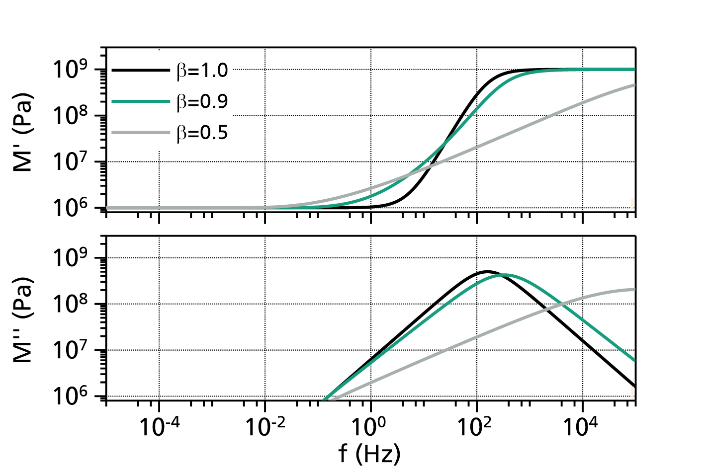
Fig. 1: Kohlrausch fit functions (with ![]() ,
, ![]() ,
, ![]() and
and ![]() ). The values for
). The values for ![]() are indicated in the legend.
are indicated in the legend.
Fig. 2: Comparison of Kohlrausch fit functions (with ![]() ,
, ![]() ,
, ![]() , and
, and ![]() ) with different viscosities
) with different viscosities ![]() . The values for
. The values for ![]() are indicated in the legend.
are indicated in the legend.
References:
Kohlrausch, R., "Theorie des elektrischen Rückstandes in der Leidner Flasche", Annalen der Physik und Chemie. 91 (1) (1854): 56–82, 179–213, doi:10.1002/andp.18541670103
Williams, G., Watts, D. C., "Non-Symmetrical Dielectric Relaxation Behavior Arising from a Simple Empirical Decay Function", Transactions of the Faraday Society 66 (1970) 80–85. doi:10.1039/tf9706600080
Kohlrausch retardation of a general modulus (circular frequency)
This function models the retardation of a general modulus (e.g. mechanical modulus) in dependence on the circular frequency ![]() with a retardation and a flow term:
with a retardation and a flow term:

The quantities are described below. It is a special case of the underlying base function with the options UseFrequencyInsteadOfOmega=false, UseFlowTerm=true, InvertViscosity=false and LogarithmizeResult=false. These options can be changed by double-clicking on the fit function.
The underlying base function models the generalized complex dynamic modulus in dependence on the circular frequency ![]() as:
as:
with the circular frequency ![]() being the independent variable (or, depending on an option, the frequency
being the independent variable (or, depending on an option, the frequency ![]() ,
, ![]() ), and
), and ![]() and
and ![]() being the dependent variables, namely the real and imaginary part of the complex dynamic modulus
being the dependent variables, namely the real and imaginary part of the complex dynamic modulus ![]() . The kernel of this equation is the Fourier transformation of the Kohlrausch function (also known as stretched exponential function, or as Kohlrausch-Williams-Watts (KWW) function).
. The kernel of this equation is the Fourier transformation of the Kohlrausch function (also known as stretched exponential function, or as Kohlrausch-Williams-Watts (KWW) function).
The typical use case is a fit to the complex dynamic mechanical modulus (e.g. shear modulus ![]() or Young's modulus
or Young's modulus ![]() ).
).
The parameters are:
- : high frequency modulus limit
- : low frequency modulus limit
- : retardation time (attention: this is not the same as the relaxation time, e.g. the maximum of is considerably shifted with respect to !)
- : shape exponent (usually ). The smaller is, the broader is the resulting frequency spectrum.
- : generalized fluidity (inverse viscosity)
- : generalized viscosity
The available options are:
UseFrequencyInsteadOfOmega:
If true, the frequency is used as the independent variable, thus in the formula above is replaced by .
If false, the circular frequency is used as the independent variable.
UseFlowTerm:
If true, the flow term in above formula is used.
If false, the flow term is not used, and the parameter corresponding with the flow term will not show in the fit.InvertViscosity:
If true, the parameter in the flow term is an inverted viscosity (i.e. fluidity). Thus the flow term generally is.
If false, the parameter in the flow term is a viscosity, and the flow term generally is.
LogarithmizeResult:
If true, the resulting values of and are logarithmized (decadic logarithm).
If false, the original values are used.
Note:
Since in most cases
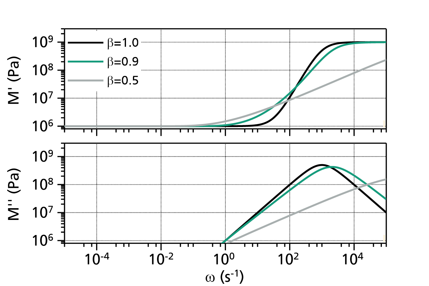
Fig. 1: Kohlrausch fit functions (with ![]() ,
, ![]() ,
, ![]() and
and ![]() ). The values for
). The values for ![]() are indicated in the legend.
are indicated in the legend.
Fig. 2: Comparison of Kohlrausch fit functions (with ![]() ,
, ![]() ,
, ![]() , and
, and ![]() ) with different viscosities
) with different viscosities ![]() . The values for
. The values for ![]() are indicated in the legend.
are indicated in the legend.
References:
Kohlrausch, R., "Theorie des elektrischen Rückstandes in der Leidner Flasche", Annalen der Physik und Chemie. 91 (1) (1854): 56–82, 179–213, doi:10.1002/andp.18541670103
Williams, G., Watts, D. C., "Non-Symmetrical Dielectric Relaxation Behavior Arising from a Simple Empirical Decay Function", Transactions of the Faraday Society 66 (1970) 80–85. doi:10.1039/tf9706600080
Havriliak-Negami retardation of a general modulus (frequency)
This function models the retardation of a general modulus (e.g. mechanical modulus) in dependence on the frequency ![]() with a retardation and a flow term:
with a retardation and a flow term:
Here, the values of the real and imaginary part of the calculated modulus are logarithmized for the output:
Should your data are not logarithmized, use a DecadicLogarithmTransformation to logarithmize them, too.
The quantities are described below. It is a special case of the underlying base function with the options UseFrequencyInsteadOfOmega=true, UseFlowTerm=true, InvertViscosity=false and LogarithmizeResult=true. These options can be changed by double-clicking on the fit function.
The underlying base function models the generalized complex dynamic modulus in dependence on the circular frequency ![]() as:
as:
with the circular frequency ![]() being the independent variable (or, depending on an option, the frequency
being the independent variable (or, depending on an option, the frequency ![]() ,
, ![]() ), and
), and ![]() and
and ![]() being the dependent variables, namely the real and imaginary part of the complex dynamic modulus
being the dependent variables, namely the real and imaginary part of the complex dynamic modulus ![]() .
.
The typical use case is a fit to the complex dynamic mechanical modulus (e.g. shear modulus ![]() or Young's modulus
or Young's modulus ![]() ).
).
The parameters are:
- : high frequency modulus limit
- : low frequency modulus limit
- : retardation time (attention: this is not the same as the relaxation time, e.g. the maximum of is considerably shifted with respect to !)
- , : shape exponents (usually and )
- : generalized fluidity (inverse viscosity)
- : generalized viscosity
The available options are:
UseFrequencyInsteadOfOmega:
If true, the frequency is used as the independent variable, thus in the formula above is replaced by .
If false, the circular frequency is used as the independent variable.
UseFlowTerm:
If true, the flow term in above formula is used.
If false, the flow term is not used, and the parameter corresponding with the flow term will not show in the fit.InvertViscosity:
If true, the parameter in the flow term is an inverted viscosity (i.e. fluidity). Thus the flow term generally is.
If false, the parameter in the flow term is a viscosity, and the flow term generally is.
LogarithmizeResult:
If true, the resulting values of and are logarithmized (decadic logarithm).
If false, the original values are used.
Note:
Since in most cases
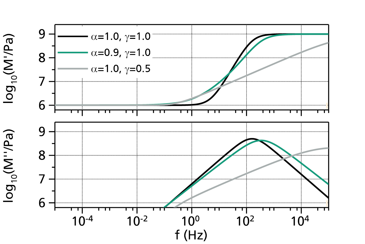
Fig. 1: Havriliak-Negami fit functions (with ![]() ,
, ![]() ,
, ![]() and
and ![]() ). The values for
). The values for ![]() and
and ![]() are indicated in the legend.
are indicated in the legend.
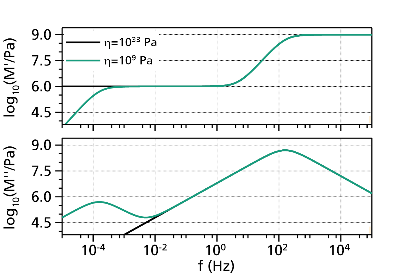
Fig. 2: Comparison of Havriliak-Negami fit functions (with ![]() ,
, ![]() ,
, ![]() ,
, ![]() and
and ![]() ) with different viscosities
) with different viscosities ![]() . The values for
. The values for ![]() are indicated in the legend.
are indicated in the legend.
References:
Havriliak, S., Negami, S., "A complex plane representation of dielectric and mechanical relaxation processes in some polymers", Polymer 8: 161–210, doi:10.1016/0032-3861(67)90021-3
Havriliak-Negami retardation of a general modulus (circular frequency)
This function models the retardation of a general modulus (e.g. mechanical modulus) in dependence on the circular frequency ![]() with a retardation and a flow term:
with a retardation and a flow term:
Here, the values of the real and imaginary part of the calculated modulus are logarithmized for the output:
Should your data are not logarithmized, use a DecadicLogarithmTransformation to logarithmize them, too.
The quantities are described below. It is a special case of the underlying base function with the options UseFrequencyInsteadOfOmega=false, UseFlowTerm=true, InvertViscosity=false and LogarithmizeResult=false. These options can be changed by double-clicking on the fit function.
The underlying base function models the generalized complex dynamic modulus in dependence on the circular frequency ![]() as:
as:
with the circular frequency ![]() being the independent variable (or, depending on an option, the frequency
being the independent variable (or, depending on an option, the frequency ![]() ,
, ![]() ), and
), and ![]() and
and ![]() being the dependent variables, namely the real and imaginary part of the complex dynamic modulus
being the dependent variables, namely the real and imaginary part of the complex dynamic modulus ![]() .
.
The typical use case is a fit to the complex dynamic mechanical modulus (e.g. shear modulus ![]() or Young's modulus
or Young's modulus ![]() ).
).
The parameters are:
- : high frequency modulus limit
- : low frequency modulus limit
- : retardation time (attention: this is not the same as the relaxation time, e.g. the maximum of is considerably shifted with respect to !)
- , : shape exponents (usually and )
- : generalized fluidity (inverse viscosity)
- : generalized viscosity
The available options are:
UseFrequencyInsteadOfOmega:
If true, the frequency is used as the independent variable, thus in the formula above is replaced by .
If false, the circular frequency is used as the independent variable.
UseFlowTerm:
If true, the flow term in above formula is used.
If false, the flow term is not used, and the parameter corresponding with the flow term will not show in the fit.InvertViscosity:
If true, the parameter in the flow term is an inverted viscosity (i.e. fluidity). Thus the flow term generally is.
If false, the parameter in the flow term is a viscosity, and the flow term generally is.
LogarithmizeResult:
If true, the resulting values of and are logarithmized (decadic logarithm).
If false, the original values are used.
Note:
Since in most cases
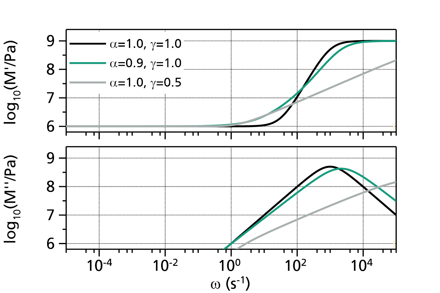
Fig. 1: Havriliak-Negami fit functions (with ![]() ,
, ![]() ,
, ![]() and
and ![]() ). The values for
). The values for ![]() and
and ![]() are indicated in the legend.
are indicated in the legend.

Fig. 2: Comparison of Havriliak-Negami fit functions (with ![]() ,
, ![]() ,
, ![]() ,
, ![]() and
and ![]() ) with different viscosities
) with different viscosities ![]() . The values for
. The values for ![]() are indicated in the legend.
are indicated in the legend.
References:
Havriliak, S., Negami, S., "A complex plane representation of dielectric and mechanical relaxation processes in some polymers", Polymer 8: 161–210, doi:10.1016/0032-3861(67)90021-3
Kohlrausch retardation of a general modulus (frequency)
This function models the retardation of a general modulus (e.g. mechanical modulus) in dependence on the frequency ![]() with a retardation and a flow term:
with a retardation and a flow term:
Here, the values of the real and imaginary part of the calculated modulus are logarithmized for the output:
Should your data are not logarithmized, use a DecadicLogarithmTransformation to logarithmize them, too.
The quantities are described below. It is a special case of the underlying base function with the options UseFrequencyInsteadOfOmega=true, UseFlowTerm=true, InvertViscosity=false and LogarithmizeResult=false. These options can be changed by double-clicking on the fit function.
The underlying base function models the generalized complex dynamic modulus in dependence on the circular frequency ![]() as:
as:
with the circular frequency ![]() being the independent variable (or, depending on an option, the frequency
being the independent variable (or, depending on an option, the frequency ![]() ,
, ![]() ), and
), and ![]() and
and ![]() being the dependent variables, namely the real and imaginary part of the complex dynamic modulus
being the dependent variables, namely the real and imaginary part of the complex dynamic modulus ![]() . The kernel of this equation is the Fourier transformation of the Kohlrausch function (also known as stretched exponential function, or as Kohlrausch-Williams-Watts (KWW) function).
. The kernel of this equation is the Fourier transformation of the Kohlrausch function (also known as stretched exponential function, or as Kohlrausch-Williams-Watts (KWW) function).
The typical use case is a fit to the complex dynamic mechanical modulus (e.g. shear modulus ![]() or Young's modulus
or Young's modulus ![]() ).
).
The parameters are:
- : high frequency modulus limit
- : low frequency modulus limit
- : retardation time (attention: this is not the same as the relaxation time, e.g. the maximum of is considerably shifted with respect to !)
- : shape exponent (usually ). The smaller is, the broader is the resulting frequency spectrum.
- : generalized fluidity (inverse viscosity)
- : generalized viscosity
The available options are:
UseFrequencyInsteadOfOmega:
If true, the frequency is used as the independent variable, thus in the formula above is replaced by .
If false, the circular frequency is used as the independent variable.
UseFlowTerm:
If true, the flow term in above formula is used.
If false, the flow term is not used, and the parameter corresponding with the flow term will not show in the fit.InvertViscosity:
If true, the parameter in the flow term is an inverted viscosity (i.e. fluidity). Thus the flow term generally is.
If false, the parameter in the flow term is a viscosity, and the flow term generally is.
LogarithmizeResult:
If true, the resulting values of and are logarithmized (decadic logarithm).
If false, the original values are used.
Note:
Since in most cases
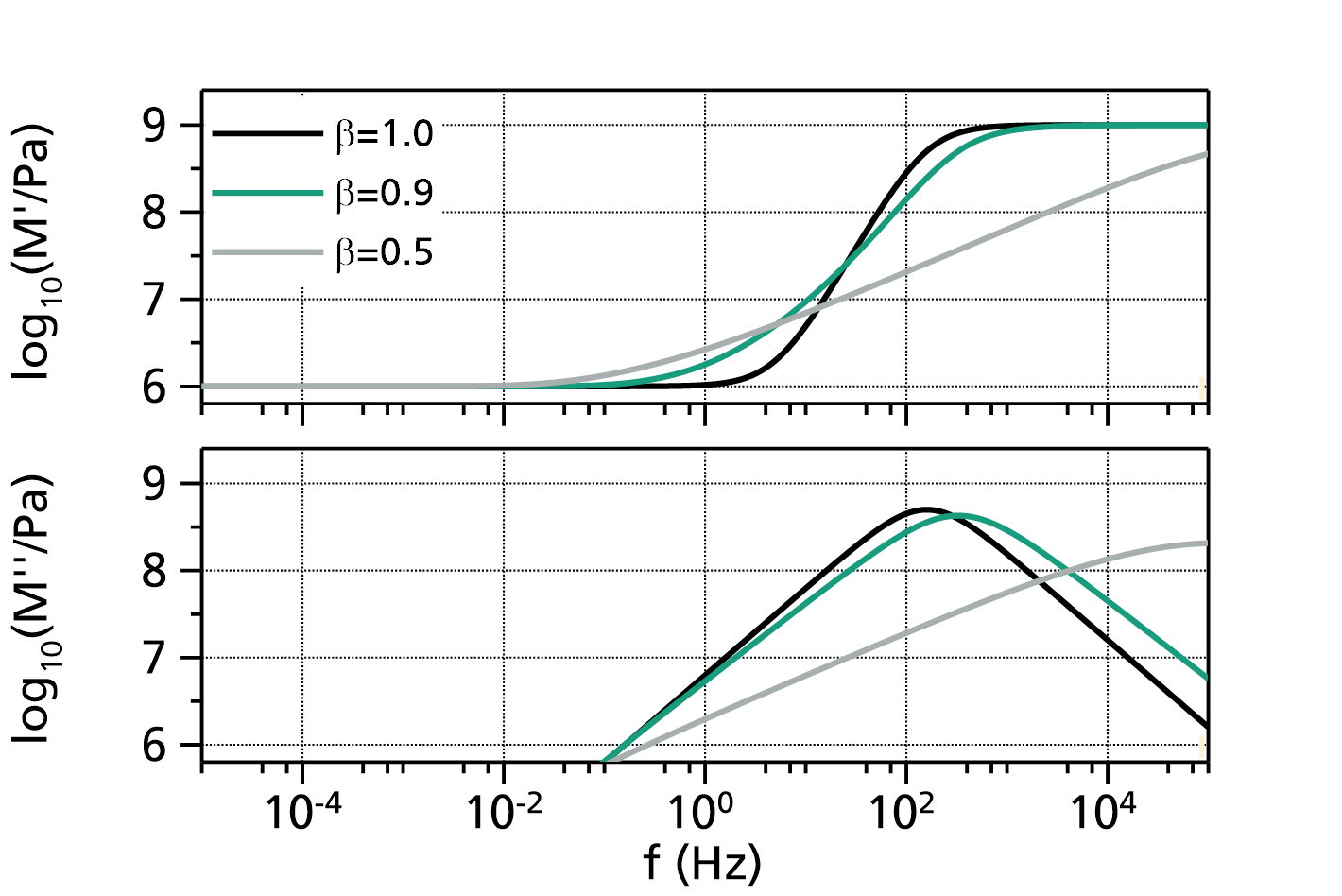
Fig. 1: Kohlrausch fit functions (with ![]() ,
, ![]() ,
, ![]() and
and ![]() ). The values for
). The values for ![]() are indicated in the legend.
are indicated in the legend.
Fig. 2: Comparison of Kohlrausch fit functions (with ![]() ,
, ![]() ,
, ![]() , and
, and ![]() ) with different viscosities
) with different viscosities ![]() . The values for
. The values for ![]() are indicated in the legend.
are indicated in the legend.
References:
Kohlrausch, R., "Theorie des elektrischen Rückstandes in der Leidner Flasche", Annalen der Physik und Chemie. 91 (1) (1854): 56–82, 179–213, doi:10.1002/andp.18541670103
Williams, G., Watts, D. C., "Non-Symmetrical Dielectric Relaxation Behavior Arising from a Simple Empirical Decay Function", Transactions of the Faraday Society 66 (1970) 80–85. doi:10.1039/tf9706600080
Kohlrausch retardation of a general modulus (circular frequency)
This function models the retardation of a general modulus (e.g. mechanical modulus) in dependence on the circular frequency ![]() with a retardation and a flow term:
with a retardation and a flow term:
Here, the values of the real and imaginary part of the calculated modulus are logarithmized for the output:
Should your data are not logarithmized, use a DecadicLogarithmTransformation to logarithmize them, too.
The quantities are described below. It is a special case of the underlying base function with the options UseFrequencyInsteadOfOmega=false, UseFlowTerm=true, InvertViscosity=false and LogarithmizeResult=false. These options can be changed by double-clicking on the fit function.
The underlying base function models the generalized complex dynamic modulus in dependence on the circular frequency ![]() as:
as:
with the circular frequency ![]() being the independent variable (or, depending on an option, the frequency
being the independent variable (or, depending on an option, the frequency ![]() ,
, ![]() ), and
), and ![]() and
and ![]() being the dependent variables, namely the real and imaginary part of the complex dynamic modulus
being the dependent variables, namely the real and imaginary part of the complex dynamic modulus ![]() . The kernel of this equation is the Fourier transformation of the Kohlrausch function (also known as stretched exponential function, or as Kohlrausch-Williams-Watts (KWW) function).
. The kernel of this equation is the Fourier transformation of the Kohlrausch function (also known as stretched exponential function, or as Kohlrausch-Williams-Watts (KWW) function).
The typical use case is a fit to the complex dynamic mechanical modulus (e.g. shear modulus ![]() or Young's modulus
or Young's modulus ![]() ).
).
The parameters are:
- : high frequency modulus limit
- : low frequency modulus limit
- : retardation time (attention: this is not the same as the relaxation time, e.g. the maximum of is considerably shifted with respect to !)
- : shape exponent (usually ). The smaller is, the broader is the resulting frequency spectrum.
- : generalized fluidity (inverse viscosity)
- : generalized viscosity
The available options are:
UseFrequencyInsteadOfOmega:
If true, the frequency is used as the independent variable, thus in the formula above is replaced by .
If false, the circular frequency is used as the independent variable.
UseFlowTerm:
If true, the flow term in above formula is used.
If false, the flow term is not used, and the parameter corresponding with the flow term will not show in the fit.InvertViscosity:
If true, the parameter in the flow term is an inverted viscosity (i.e. fluidity). Thus the flow term generally is.
If false, the parameter in the flow term is a viscosity, and the flow term generally is.
LogarithmizeResult:
If true, the resulting values of and are logarithmized (decadic logarithm).
If false, the original values are used.
Note:
Since in most cases
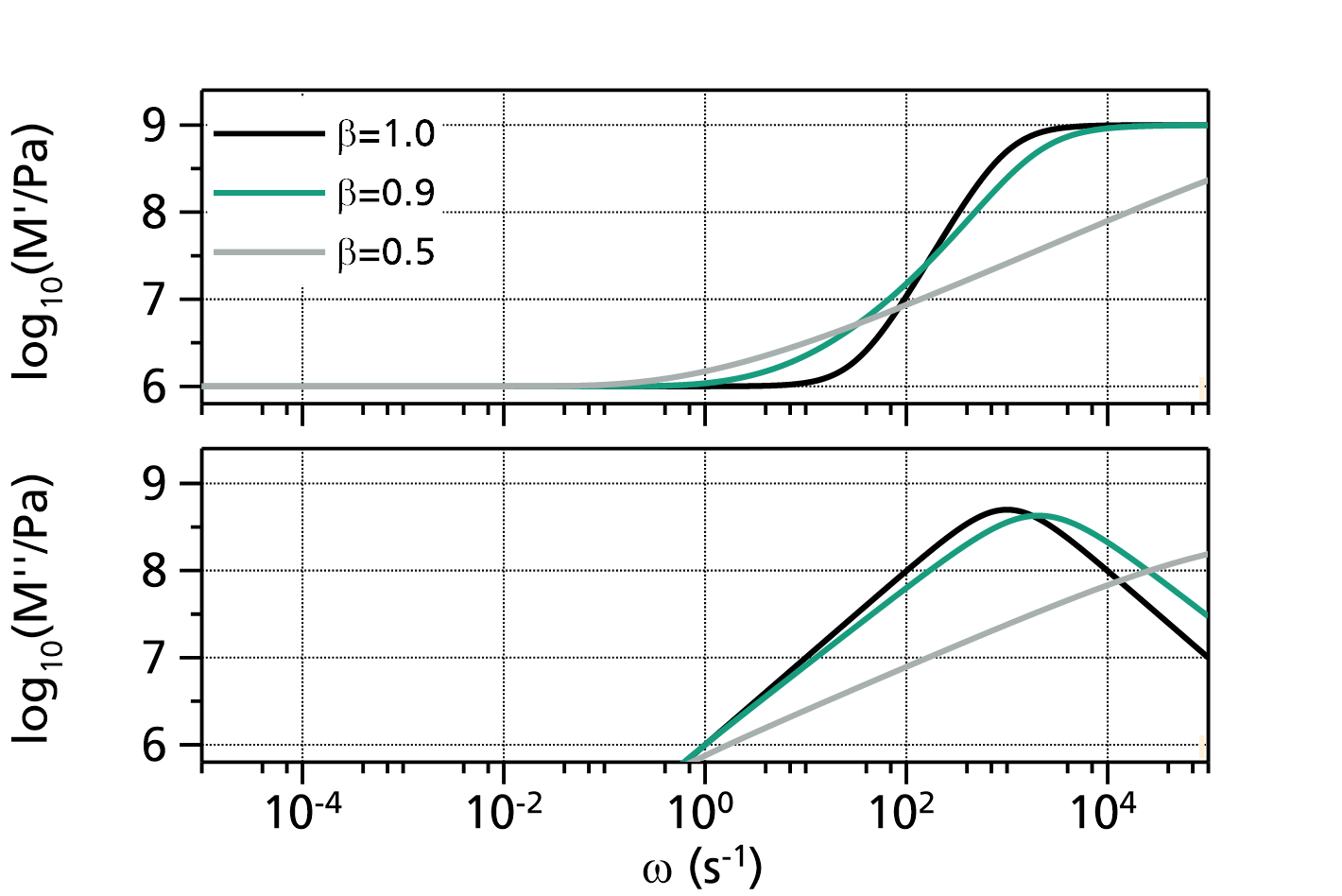
Fig. 1: Kohlrausch fit functions (with ![]() ,
, ![]() ,
, ![]() and
and ![]() ). The values for
). The values for ![]() are indicated in the legend.
are indicated in the legend.
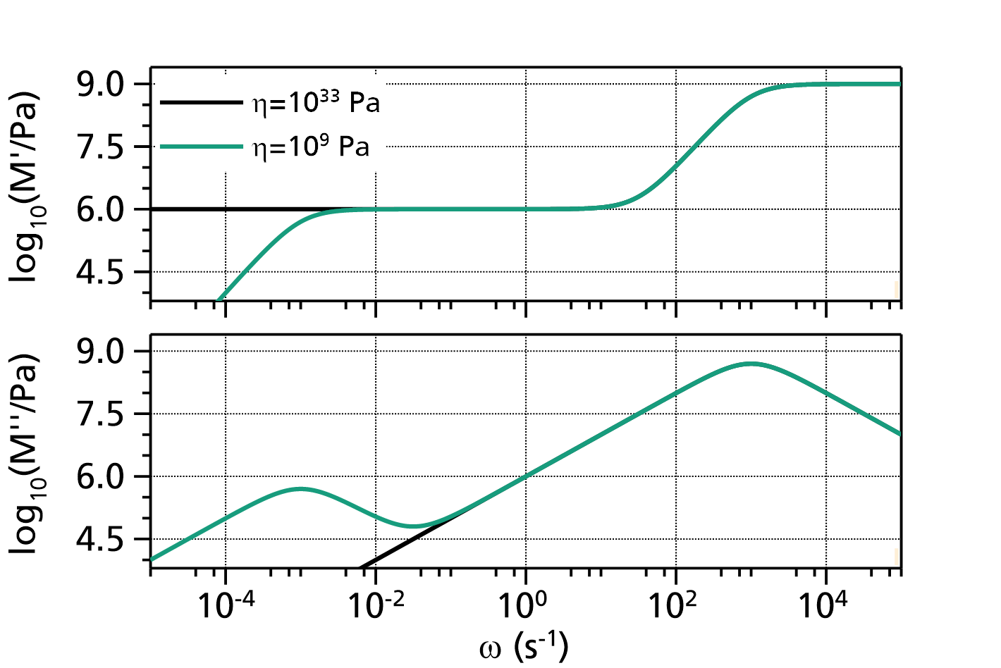
Fig. 2: Comparison of Kohlrausch fit functions (with ![]() ,
, ![]() ,
, ![]() , and
, and ![]() ) with different viscosities
) with different viscosities ![]() . The values for
. The values for ![]() are indicated in the legend.
are indicated in the legend.
References:
Kohlrausch, R., "Theorie des elektrischen Rückstandes in der Leidner Flasche", Annalen der Physik und Chemie. 91 (1) (1854): 56–82, 179–213, doi:10.1002/andp.18541670103
Williams, G., Watts, D. C., "Non-Symmetrical Dielectric Relaxation Behavior Arising from a Simple Empirical Decay Function", Transactions of the Faraday Society 66 (1970) 80–85. doi:10.1039/tf9706600080
ErrorFunctionFromTo
This function evaluates a smooth transition between two polynomial segments, using the error function [1], according to:
in which:
 is the error function
 is the x-coordinate of the transition point
- is the width of the transition
- is the y-coordinate of the point at which the two polynomial segments are joined
- are the polynomial coefficients of the left polynomial (small x values)
- ... are the polynomial coefficients of the right polynomial(large x values)
- is the order of the left polynomial ()
- is the order of the right polynomial ()
The polynomial orders ![]() and
and ![]() can be changed by double-clicking on the fit function. The default values are
can be changed by double-clicking on the fit function. The default values are ![]() and
and ![]() , resulting in a smooth transition between two constant levels at the center position
, resulting in a smooth transition between two constant levels at the center position ![]() .
.
The domain of the function generally is ![]() . If both polynomial orders are zero, then the domain of the function is
. If both polynomial orders are zero, then the domain of the function is ![]() .
.
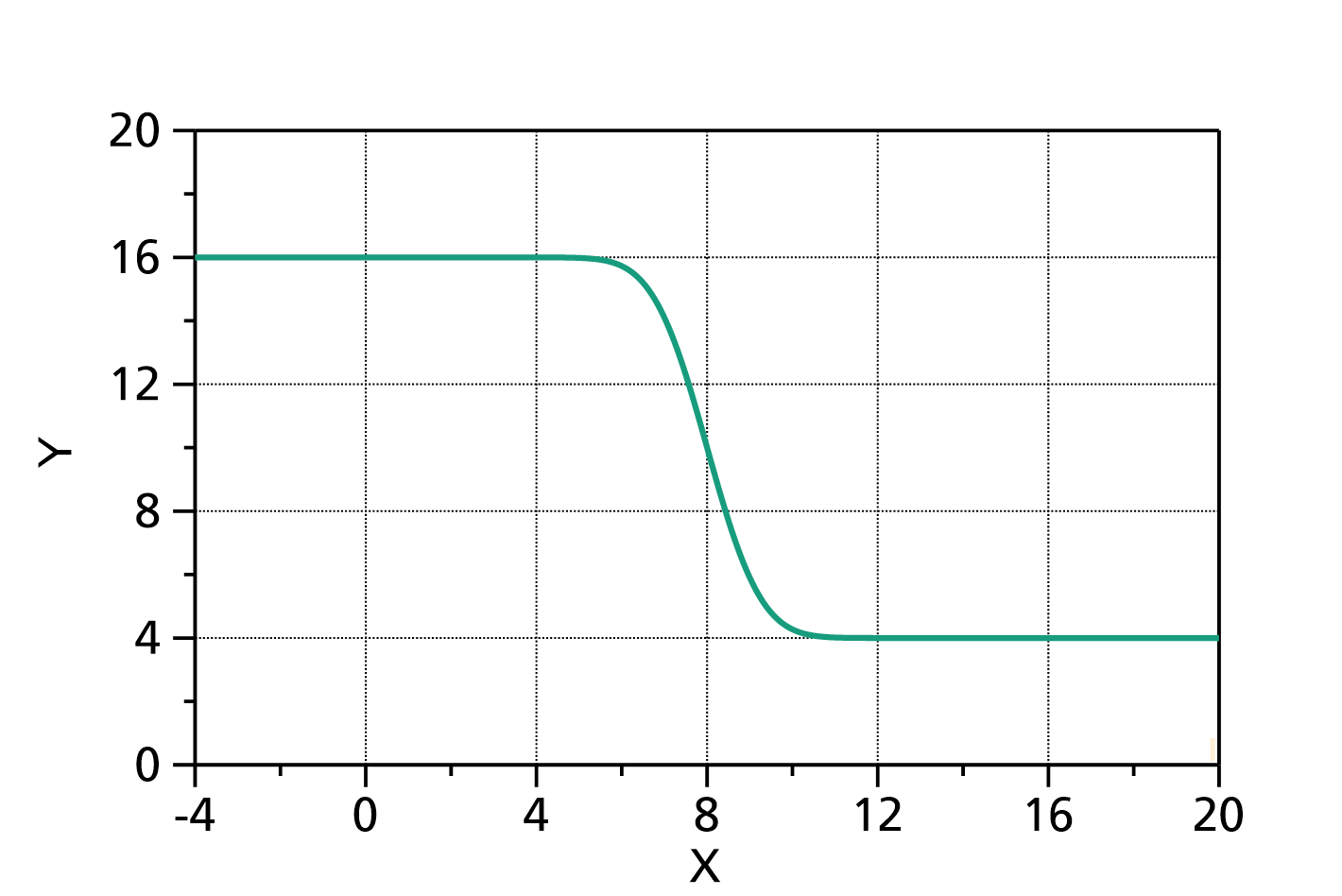
Fig. 1: ErrorFunctionFromTo (![]() ,
, ![]() ) with
) with ![]() ,
, ![]() ,
, ![]() and
and ![]() .
.
Literature:
[1] Error function in Wikipedia
General effective medium transition
This transition models e.g. the DC electrical conductivity of conductive particles embedded in a matrix, but is also suitable for other percolation problems.
The function, which evaluates the property ![]() of a compound in dependence of a filler concentration
of a compound in dependence of a filler concentration ![]() (
(![]() ) is implicitly given by the following equation:
) is implicitly given by the following equation:

in which:
 : volume concentration of the filler particles (
 )
)
 : critical percolation threshold (location of the transition (
 ))
))
 : exponents (
 ,
,  )
)
- : property of the matrix material (e.g. electrical conductivity of the matrix)
 : property of the filler particles (e.g. electrical conductivity of the filler)
- : resulting property of the compound (e.g. electrical conductivity of the matrix with filler particles)
The equation has the following properties, which match the percolation theory for concentrations below and above the percolation threshold:
 for
for 
 for
for 
 for
for 
 for
for 
In contrast to the separate percolation equations below and above the percolation threshold, the general effective medium transition avoids the divergence near the percolation threshold, and provides a smooth transition between the two equations.

Fig. 1: GeneralEffectiveMedium transition with ![]() ,
, ![]() ,
, ![]() ,
, ![]() and
and ![]() .
.
References:
McLachlan, D. and G. Sauti. “The AC and DC conductivity of nanocomposites.” Journal of Nanomaterials 2007 (2007): 15, doi:10.1155/2007/30389
GeneralizedLogisticDecreasing
This function evaluates a sum of generalized logistic terms (decreasing steps), plus a background polynomial with one or multiple terms, according to
in which:
- are the amplitudes (step heights) of the logistic step terms
- are the locations of the logistic step terms
- are the widths of the logistic step terms
- are exponents that control the slope (steepness) on the left sides of the steps
 are exponents that control the slope (steepness) on the right sides of the steps
- are the coefficients of the background polynomial of order
- is the number of logistic step terms ()
- is the order of the background polynomial (set to disable the background polynomial)
The number of logistic step terms ![]() and the order of the background polynomial
and the order of the background polynomial ![]() can be changed by double-clicking on the fit function. The default values are
can be changed by double-clicking on the fit function. The default values are ![]() and
and ![]() .
.
The domain of the function is ![]() .
.
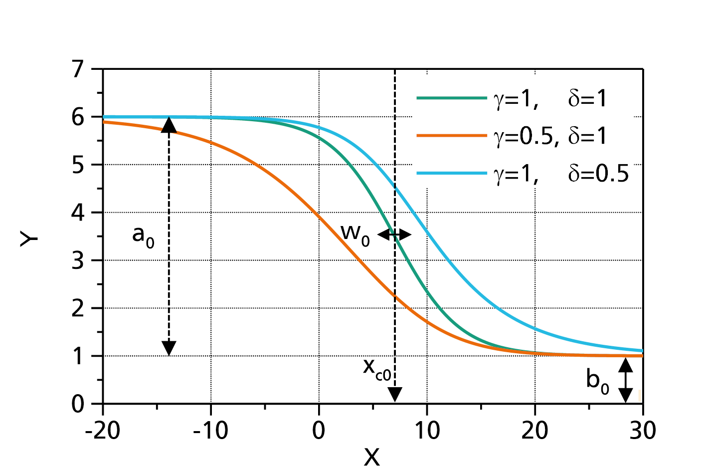
Fig. 1: GeneralizedLogisticDecreasing (![]() ,
, ![]() ) with
) with ![]() ,
, ![]() ,
, ![]() and
and ![]() . The values of
. The values of ![]() and
and ![]() are indicated in the legend.
are indicated in the legend.
References: Sigmoid function at Wikipedia
GeneralizedLogisticIncreasing
This function evaluates a sum of generalized logistic terms (increasing steps), plus a background polynomial with one or multiple terms, according to
in which:
- are the amplitudes (step heights) of the logistic step terms
- are the locations of the logistic step terms
- are the widths of the logistic step terms
- are exponents that control the slope (steepness) on the right sides of the steps
- are exponents that control the slope (steepness) on the left sides of the steps
- are the coefficients of the background polynomial of order
- is the number of logistic step terms ()
- is the order of the background polynomial (set to disable the background polynomial)
The number of logistic step terms ![]() and the order of the background polynomial
and the order of the background polynomial ![]() can be changed by double-clicking on the fit function. The default values are
can be changed by double-clicking on the fit function. The default values are ![]() and
and ![]() .
.
The domain of the function is ![]() .
.
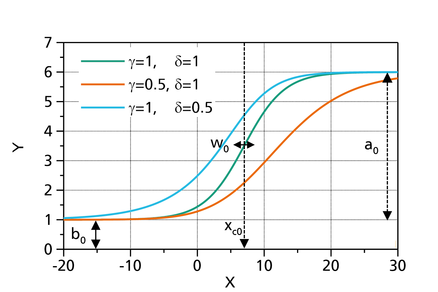
Fig. 1: GeneralizedLogisticIncreasing (![]() ,
, ![]() ) with
) with ![]() ,
, ![]() ,
, ![]() and
and ![]() . The values of
. The values of ![]() and
and ![]() are indicated in the legend.
are indicated in the legend.
References: Sigmoid function at Wikipedia
Gompertz function / transition
The Gompertz function is used in biology to describe growth rates of cells and mortality [1].
This fit function evaluates a smooth transition between two polynomial segments, using the Gompertz function, according to:
in which:
x is the independent variable (for growth description, this is time)
- is the x-coordinate of the transition point (
 part)
part)
- is the growth rate
- is the y-coordinate of the point at which the two polynomial segments are joined
- are the polynomial coefficients of the left polynomial (small x values)
- ... are the polynomial coefficients of the right polynomial(large x values)
- is the order of the left polynomial ()
- is the order of the right polynomial ()
The polynomial orders ![]() and
and ![]() can be changed by double-clicking on the fit function. The default values are
can be changed by double-clicking on the fit function. The default values are ![]() and
and ![]() , resulting in a smooth transition between two constant levels at the center position
, resulting in a smooth transition between two constant levels at the center position ![]() .
.
The domain of the function generally is ![]() . If both polynomial orders are zero, then the domain of the function is
. If both polynomial orders are zero, then the domain of the function is ![]() .
.
If ![]() and
and ![]() , one gets the Gompertz function that is described in [1], with
, one gets the Gompertz function that is described in [1], with ![]() being the asymptote for
being the asymptote for ![]() .
.
Fig. 1: Gompertz function (![]() ,
, ![]() ) with
) with ![]() ,
, ![]() ,
, ![]() and
and ![]() .
.
References:
[1] Gompertz function in Wikipedia
General effective medium transition (logarithmized)
This transition models e.g. the DC electrical conductivity of conductive particles embedded in a matrix, but is also suitable for other percolation problems.
The function, which evaluates the property ![]() of a compound in dependence of a filler concentration
of a compound in dependence of a filler concentration ![]() (
(![]() ) is implicitly given by the following equation:
) is implicitly given by the following equation:
in which:
- : volume concentration of the filler particles ()
- : critical percolation threshold (location of the transition ())
- : exponents (, )
- : property of the matrix material (e.g. electrical conductivity of the matrix)
- : property of the filler particles (e.g. electrical conductivity of the filler)
- : resulting property of the compound (e.g. electrical conductivity of the matrix with filler particles)
Instead of returning ![]() as described above, the function will return the decadic logarithm
as described above, the function will return the decadic logarithm ![]() . Furthermore, instead of
. Furthermore, instead of ![]() and
and ![]() , the logarithmized parameters
, the logarithmized parameters ![]() and
and ![]() are used!
are used!
The equation has the following properties, which match the percolation theory for concentrations below and above the percolation threshold:
- for
- for
- for
- for
In contrast to the separate percolation equations below and above the percolation threshold, the general effective medium transition avoids the divergence near the percolation threshold, and provides a smooth transition between the two equations.
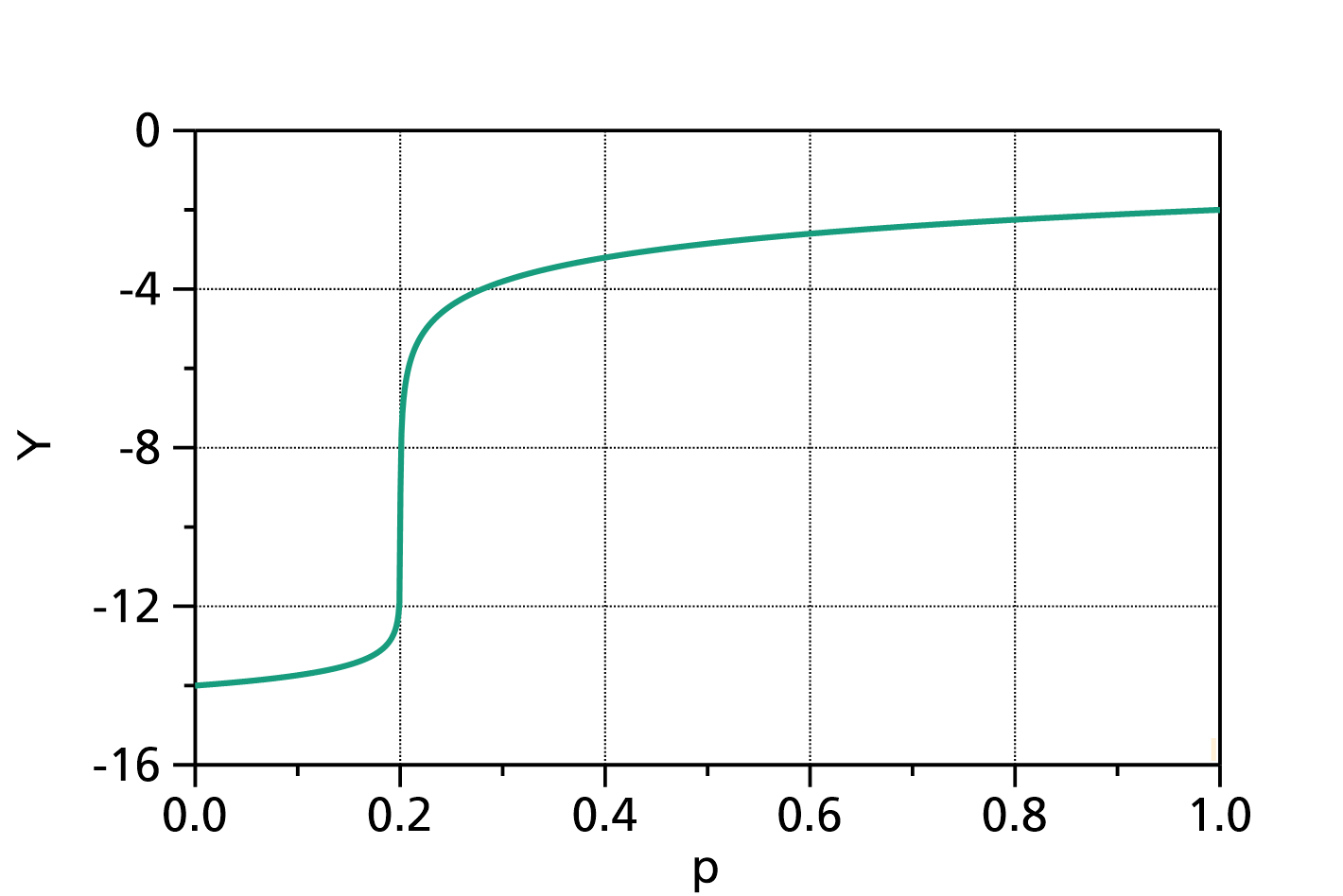
Fig. 1: Lg10GeneralEffectiveMedium transition with the parameters ![]() ,
, ![]() ,
, ![]() ,
, ![]() and
and ![]() .
.
References:
McLachlan, D. and G. Sauti. “The AC and DC conductivity of nanocomposites.” Journal of Nanomaterials 2007 (2007): 15, doi:10.1155/2007/30389
Linear Fermi-Dirac transition
This fit function implements the linearly scaled Fermi-Dirac transition:
which assumes a value of ![]() for
for ![]() and
and ![]() for
for ![]() .
.
The core ![]() of the Fermi-Dirac transition is the following function, defined in the interval
of the Fermi-Dirac transition is the following function, defined in the interval ![]() , which assumes the values
, which assumes the values ![]() and
and ![]() :
:
in which:
- : location of the transition (0..1)
 : width parameter
The domain of the function is ![]() .
.
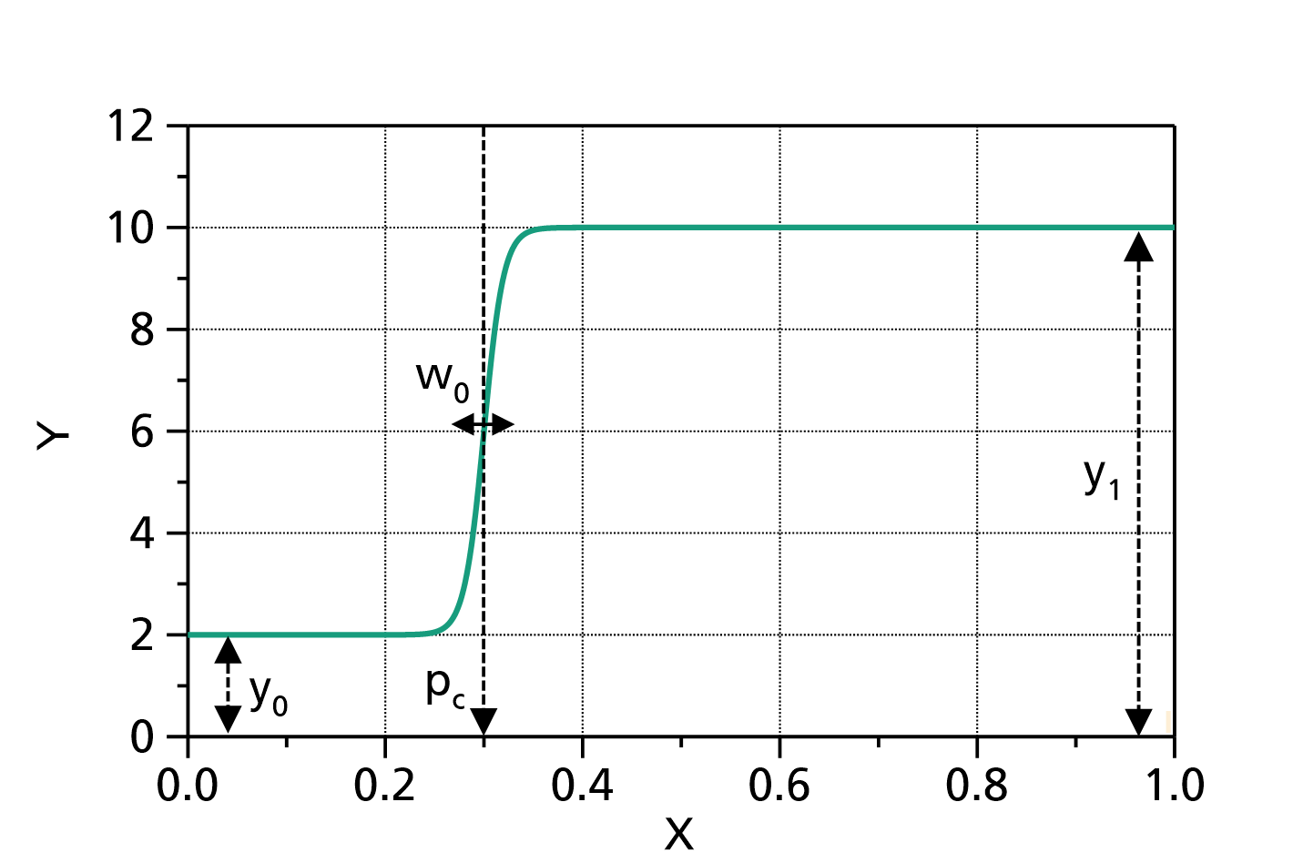
Fig. 1: LinearFermiDiracTransition with ![]() ,
, ![]() ,
, ![]() and
and ![]() .
.
References:
Logarithmic Fermi-Dirac transition
This fit function implements the linearly scaled Fermi-Dirac transition:
which assumes a value of ![]() for
for ![]() and
and ![]() for
for ![]() . It is used e.g. to model the behavior of electrical conductivity in dependence on the concentration
. It is used e.g. to model the behavior of electrical conductivity in dependence on the concentration ![]() and the critical concentration
and the critical concentration ![]() (percolation behavior).
(percolation behavior).
The core ![]() of the Fermi-Dirac transition is the following function, defined in the interval
of the Fermi-Dirac transition is the following function, defined in the interval ![]() , which assumes the values
, which assumes the values ![]() and
and ![]() :
:
in which:
- : location of the transition (0..1)
- : width parameter
The domain of the function is ![]() .
.
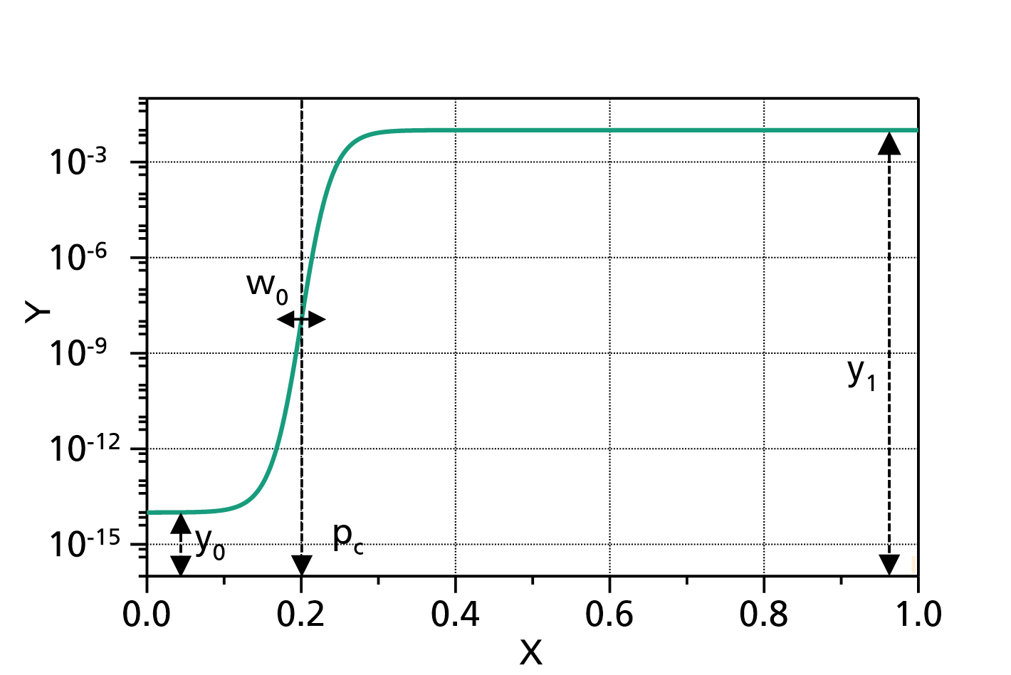
Fig. 1: LogarithmicFermiDiracTransition with ![]() ,
, ![]() ,
, ![]() and
and ![]() . This could e.g. be a typical curve for the electrical conductivity of a carbon black filled composite in dependence on the carbon black volume concentration.
. This could e.g. be a typical curve for the electrical conductivity of a carbon black filled composite in dependence on the carbon black volume concentration.
References:
LogisticDecreasing
This function evaluates a sum of logistic terms (decreasing steps), plus a background polynomial with one or multiple terms, according to
in which:
- are the amplitudes (step heights) of the logistic step terms
- are the locations of the logistic step terms
- are the widths of the logistic step terms
- are the coefficients of the background polynomial of order
- is the number of logistic step terms ()
- is the order of the background polynomial (set to disable the background polynomial)
The number of logistic step terms ![]() and the order of the background polynomial
and the order of the background polynomial ![]() can be changed by double-clicking on the fit function. The default values are
can be changed by double-clicking on the fit function. The default values are ![]() and
and ![]() .
.
The domain of the function is ![]() .
.
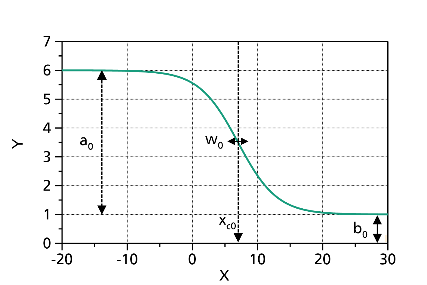
Fig. 1: LogisticDecreasing (![]() ,
, ![]() ) with
) with ![]() ,
, ![]() ,
, ![]() and
and ![]() .
.
References: Sigmoid function at Wikipedia
LogisticIncreasing
This function evaluates a sum of logistic terms (increasing steps), plus a background polynomial with one or multiple terms, according to
in which:
- are the amplitudes (step heights) of the logistic step terms
- are the locations of the logistic step terms
- are the widths of the logistic step terms
- are the coefficients of the background polynomial of order
- is the number of logistic step terms ()
- is the order of the background polynomial (set to disable the background polynomial)
The number of logistic step terms ![]() and the order of the background polynomial
and the order of the background polynomial ![]() can be changed by double-clicking on the fit function. The default values are
can be changed by double-clicking on the fit function. The default values are ![]() and
and ![]() .
.
The domain of the function is ![]() .
.
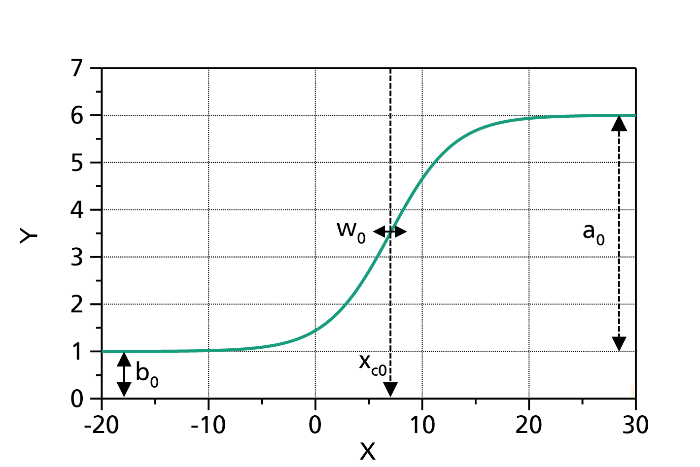
Fig. 1: LogisticIncreasing (![]() ,
, ![]() ) with
) with ![]() ,
, ![]() ,
, ![]() and
and ![]() .
.
References: Sigmoid function at Wikipedia
Smoothed percolation
The base of this function are the two percolation equations valid below and above the percolation threshold ![]() :
:
- for (left side equation)}
- for (right side equation)
in which:
- : critical percolation threshold (location of the transition (0..1))
- : volume concentration of the filler particles (0..1)
- : exponents (, )
- : property of the matrix (e.g. electrical conductivity of the matrix,
 )
)
- : property of the filler particles (e.g. electrical conductivity of the filler,
 )
)
- : resulting property of the compound (e.g. electrical conductivity of the matrix with filler particles)
Because both equations diverge at ![]() , we need to smooth that location.
For this we use somewhat stricter boundaries:
, we need to smooth that location.
For this we use somewhat stricter boundaries:
Calculate the approximate logarithmic step height of the transition by
Find a
 such that the quotient of the function values of right side and left side approximately match this step height:

in which ![]() (obviously:
(obviously: ![]() ).
).
The value of ![]() is then used as the upper boundary of the left side percolation equation:
is then used as the upper boundary of the left side percolation equation:
![]() for
for ![]()
and the value of ![]() is used as the lower boundary of the right side percolation equation:
is used as the lower boundary of the right side percolation equation:
![]() for
for ![]()
In the interval between ![]() and
and ![]() , the function values are approximated by a logarithmic function:
, the function values are approximated by a logarithmic function:
![]()
in which
- value of as evaluated by the left side equation at

 value of as evaluated by the right side equation at
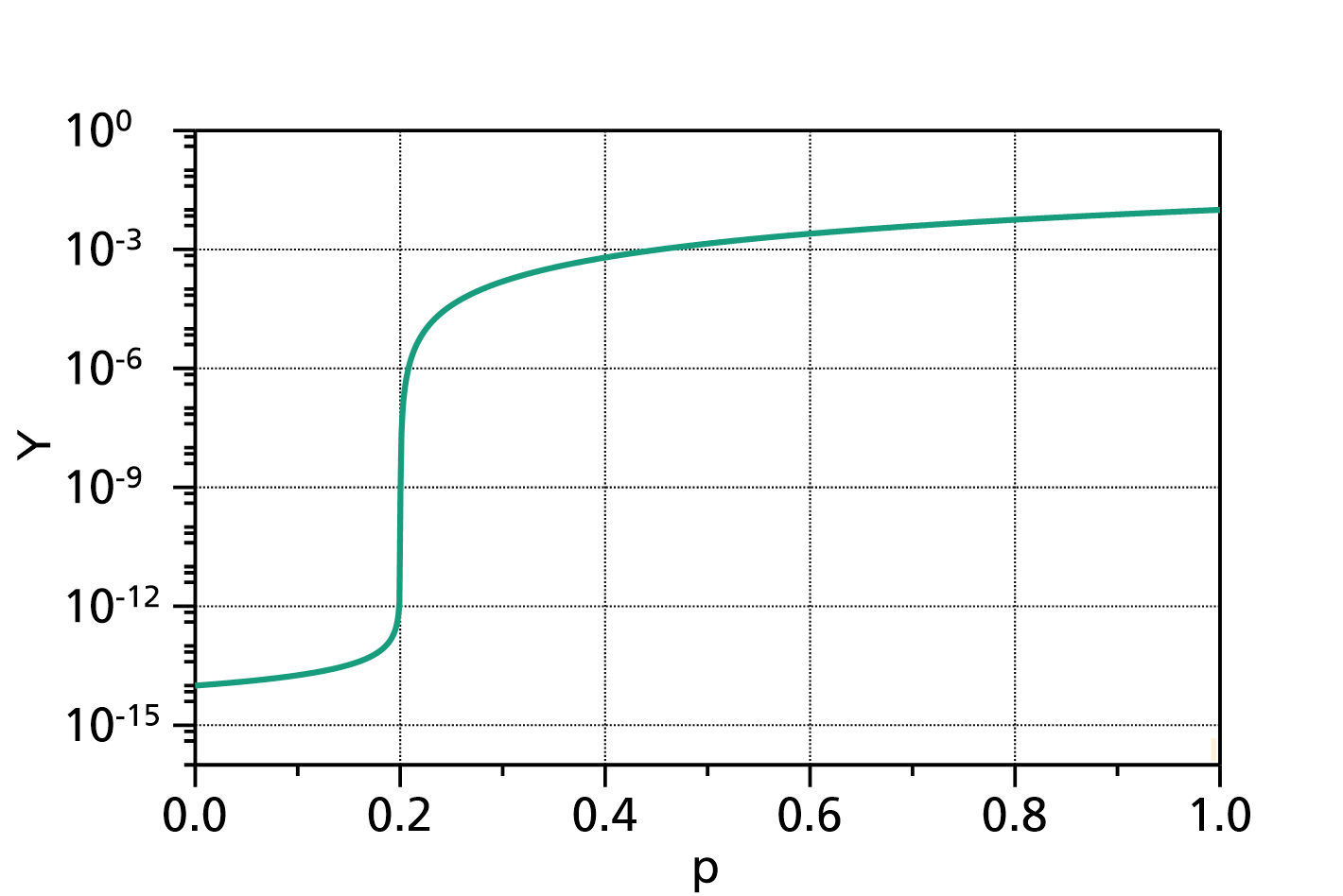
Fig. 1: SmoothedPercolation transition with ![]() ,
, ![]() ,
, ![]() ,
, ![]() and
and ![]() .
.
Bingham plastic model
This model describes the dependence of the viscosity ![]() on the shear rate
on the shear rate ![]() according to the following equation:
according to the following equation:
in which:
- : yield stress
 : viscosity (limes for high shear rates)
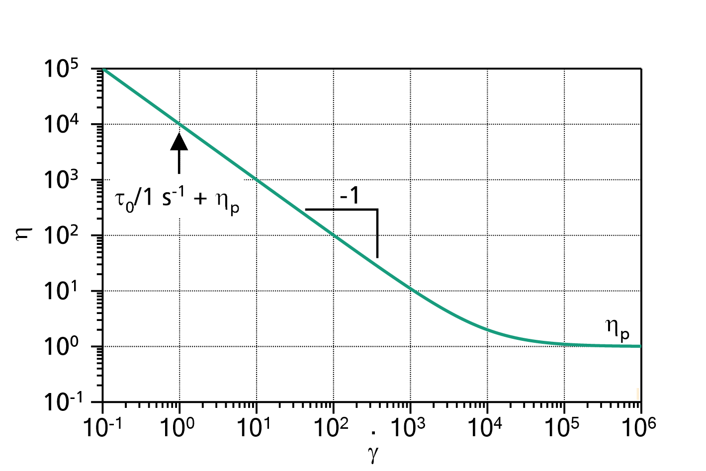
Fig. 1: Bingham plastic model with ![]() and
and ![]() .
.
References:
Bingham, E.C. (1916). "An Investigation of the Laws of Plastic Flow". Bulletin of the Bureau of Standards. 13 (2): 309–353. doi:10.6028/bulletin.304. hdl:2027/mdp.39015086559054
Carreau-Yasuda model
This model describes the dependence of the viscosity ![]() on the shear rate
on the shear rate ![]() according to the following equation:
according to the following equation:
in which:
 : zero shear viscosity
 : terminal viscosity at very high shear rates (
 )
)
 : parameter (inverse characteristic viscosity)
 , : exponents (
 ,
,  )
)
In the special case ![]() this model is equivalent to the Cross model.
this model is equivalent to the Cross model.
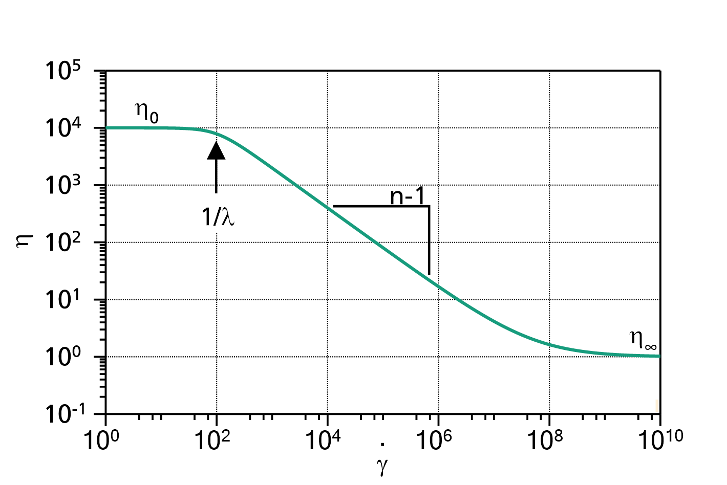
Fig. 1: Carreau-Yasuda model with ![]() ,
, ![]() ,
, ![]() ,
, ![]() and
and ![]() .
.
References:
Yasuda K, Armstrong RC, Cohen RE (1981) Shear flow properties of concentrated solutions of linear and star branched polystyrenes. Rheol Acta 20:163–178
Cross model
This model describes the dependence of the viscosity ![]() on the shear rate
on the shear rate ![]() according to the following equation:
according to the following equation:
in which:
- : zero shear viscosity
- : terminal viscosity at very high shear rates ()
 : parameters,
  ,
,
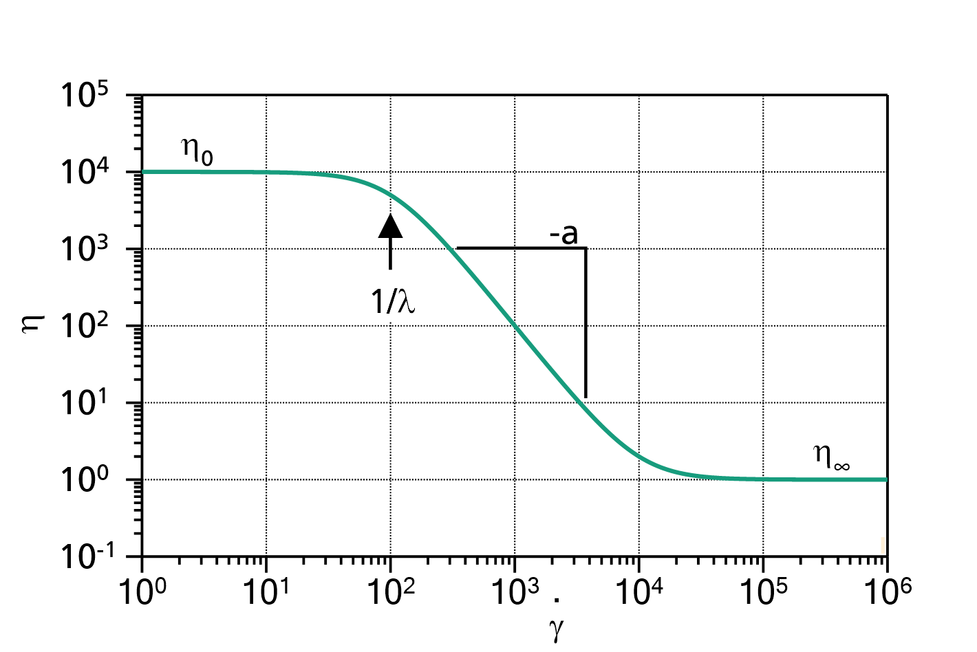
Fig. 1: Cross model with ![]() ,
, ![]() ,
, ![]() and
and ![]() .
.
References:
Cross MM (1965) Rheology of non-Newtonian fluids—a new flow equation for pseudoplastic systems. J Colloid Sci 20:417–437
Cross MM (1979) Relation between viscoelasticity and shear-thinning behaviour in liquids. Rheol Acta 18:609–614
Herschel-Bulkley model
This model describes the dependence of the viscosity ![]() on the shear rate
on the shear rate ![]() according to the following equation:
according to the following equation:
in which:
- : yield stress
- : pre-factor
- : exponent ()
Note: With
this model is equivalent to the Bingham plastic model.
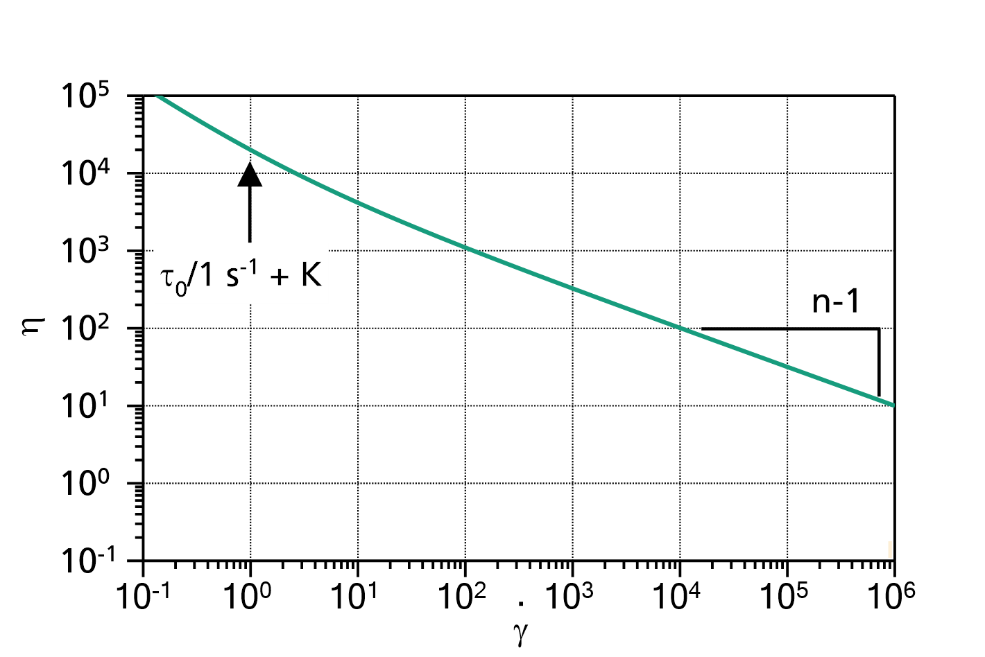
Fig. 1: Herschel-Bulkley model with ![]() ,
, ![]() and
and ![]() .
.
References:
Herschel, W.H.; Bulkley, R. (1926), "Konsistenzmessungen von Gummi-Benzollösungen", Kolloid Zeitschrift, 39 (4): 291–300, doi:10.1007/BF01432034, S2CID 97549389
Power law model
This model describes the dependence of the viscosity ![]() on the shear rate
on the shear rate ![]() according to the following equation:
according to the following equation:
in which:
- : pre-factor
- : exponent ()
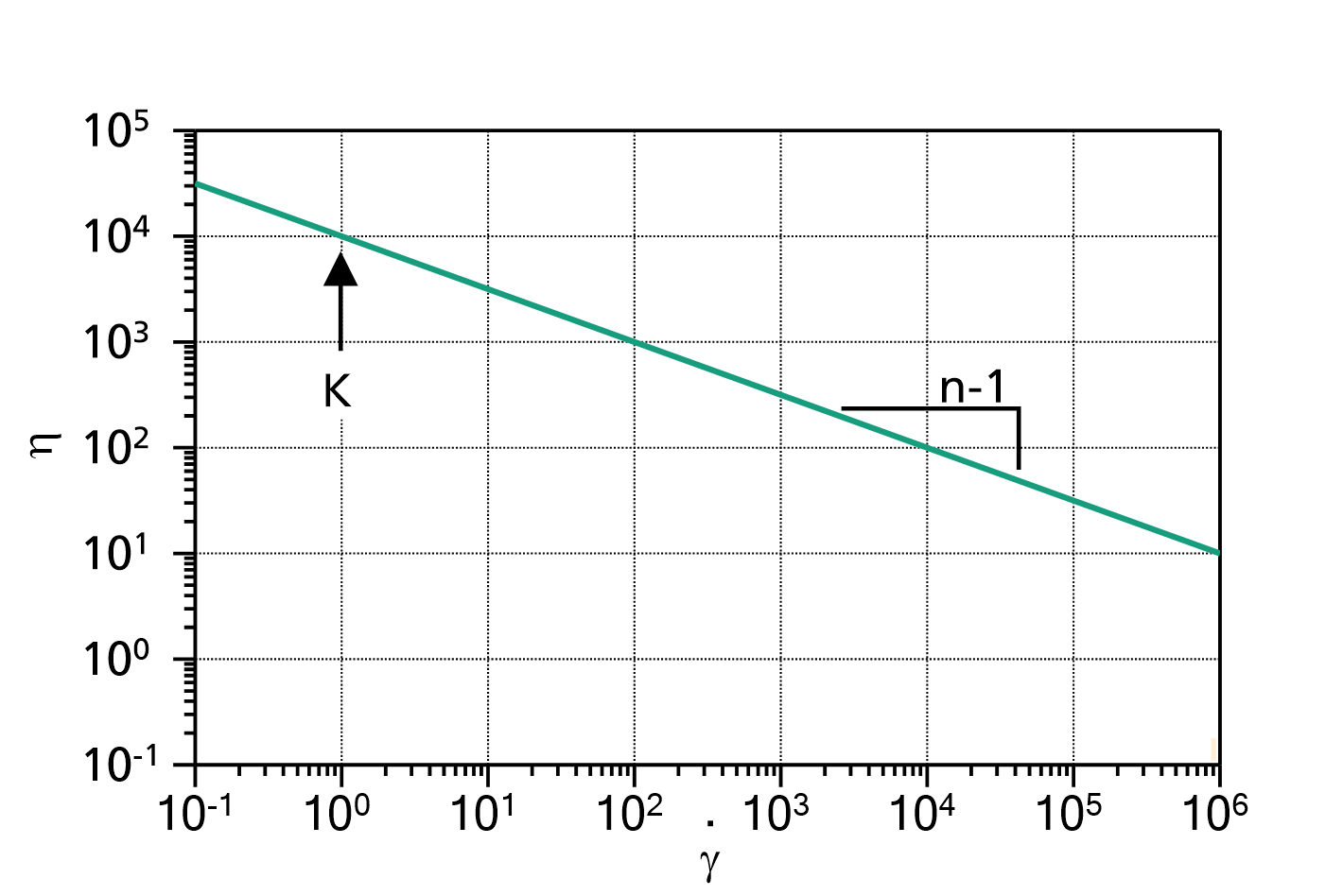
Fig. 1: Power law model with ![]() and
and ![]() .
.
References:
Markus Reiner et al., "Viskosimetrische Untersuchungen an Lösungen hochmolekularer Naturstoffe", Kolloid Zeitschrift (1933) 65 (1) 44-62
Next section: Altaxo's command line arguments